Inertial Sensor Allan Variance Characterization Methods
Allan variance isolates sensor white noise, flicker floor, and random walk by evaluating cluster time variances on an isolated seismic bench.

Anchor
Allan variance resolves the time-domain stochastic structure of an inertial sensor into distinct noise processes by mapping variance against cluster integration time. A single static run gives a buyer the white noise floor, the flicker floor, and the random run-to-run walk coefficients needed to populate a navigation filter. The test demands physical stillness.
A turntable isolation pad must attenuate ambient ground motion below the micro-g threshold across the entire recording window. When high-frequency seismic noise leaks into an accelerometer dataset, the short-cluster averaging region distorts immediately. The engineer reads an elevated velocity random walk coefficient that belongs to the facility floor rather than the silicon proof mass.
Thermal stability matters equally. A room temperature swing of two degrees Celsius over twenty-four hours drives low-frequency drift that masquerades as rate random walk on a gyroscopic trace.
Ambient seismic displacement above two hundred nanometers per second corrupts angle random walk extraction on navigation-grade instruments.
Inertial sensor characterization rests on capturing long, uncorrupted records of zero-rate and zero-specific-force output. The IEEE-standardized Allan variance formulation splits these continuous records into consecutive bins of duration tau. Averaging the instantaneous rate or acceleration within each bin, subtracting adjacent bin averages, and calculating the sample variance of those differences yields the Allan deviation plot.
The resulting curve traces the sensor noise profile from wideband thermal noise down through 1/f flicker limits to environmental trending. The engineer separates intrinsic sensor electronics from external laboratory interference by evaluating the characteristic slopes on log-log axes.
Suppliers frequently publish angle random walk derived from power spectral density integration while omitting the flicker floor. When this occurs, the buyer receives a part that looks compliant over a two-second integration window but drifts unboundedly inside an operational Kalman filter across twenty minutes. Characterization procedures isolate these discrete stochastic regimes to eliminate procurement surprises.

Arithmetic
Processing an inertial time series begins with the continuous integration of the sensor output rate into an angle, or acceleration into a velocity. Let the discrete output sequence sampled at interval tau-zero be represented by discrete readings across total points N. Forming cluster intervals of duration tau, equal to m times tau-zero, produces grouped data blocks. The standard Allan variance expression calculates the difference between adjacent cluster averages, squaring the results and taking the expected value across the full record duration.
Overlapping Allan variance alters this basic cluster routine. Rather than stepping the cluster window forward by its full length tau, the overlapping algorithm steps forward by a single sample period tau-zero. The arithmetic expands the statistical degrees of freedom dramatically for larger values of tau, narrowing the confidence intervals of the estimator without increasing laboratory logging time.
For a dataset of N discrete samples, the overlapping variance estimator processes all possible clusters of length m:
sigma squared of tau equals one divided by two times m squared times tau-zero squared times the quantity N minus two m, multiplied by the summation from k equals one to N minus two m of the squared second difference of the discrete angle coordinate sequence. The overlapping variance produces tighter estimation bands at long integration periods, resolving bias instability minimums that non-overlapping calculations leave obscured by statistical scattering.
Modified Allan variance introduces an additional phase-averaging operation across the cluster samples before calculating the second differences. This algorithmic variation separates white phase noise from flicker phase noise. Standard Allan variance produces an identical slope of negative one on a log-log plot for both mechanisms, creating ambiguity when evaluating capacitive pick-off preamplifiers.
Modified Allan variance forces white phase noise to assume a slope of negative one point five, leaving flicker phase noise at a slope of negative one.
Which Processing Mode Isolates True Instrument Drift?
The standard overlapping Allan variance remains the industrial reference for rate gyroscopes and linear accelerometers when extracting navigation error parameters. Dynamic Allan variance evaluates non-stationary time series by sweeping a sliding time-window along the temporal record, generating a three-dimensional surface of noise coefficients against elapsed experiment time. This method flags transient thermal settling, die-attach stress relaxation, and voltage reference degradation during the early burn-in phase of an inertial measurement unit.
| Noise Mechanism | Log-Log Slope | Rate Gyroscope Units | Accelerometer Units | Extraction Point |
|---|---|---|---|---|
| Quantization Noise | -1.0 | arcsec | m/s | tau equals square root of 3 |
| Angle / Velocity Random Walk | -0.5 | deg / root-hour | m/s / root-hour | tau equals 1 second |
| Bias Instability (Flicker) | 0.0 | deg / hour | micro-g | Curve flat minimum / 0.664 |
| Rate / Accel Random Walk | +0.5 | deg / hour / root-hour | micro-g / root-hour | tau equals 3 seconds |
| Ramp Drift (Systematic) | +1.0 | deg / hour squared | micro-g / hour | tau equals square root of 2 |
The extraction of coefficients follows strict geometric rules on the log-log plane. Angle random walk emerges from the negative zero-point-five slope line evaluated at an integration time of one second. Bias instability occupies the flat minimum where the curve slope crosses zero, requiring a divisor of zero point six six four derived from the logarithmic integration of a 1/f power spectral density over a finite window.
Rate random walk appears along the positive zero-point-five slope line, extracted at an integration time of three seconds. Systematic linear acceleration drift creates a steep positive slope of plus one, intersecting the curve at an integration time of the square root of two.
IEEE Std 952 details the extraction geometry for gyroscopes, while IEEE Std 1293 establishes the matching parameters for linear single-axis accelerometers.
Rig
Mechanical mounting isolates the device under test from environmental culture. A granite surface table resting on pneumatic vibration isolators provides the baseline floor. The natural frequency of the passive air bladders must sit between one point two and two point zero hertz.
Air-handling ducts within the test facility introduce acoustic energy between sixty and one hundred twenty hertz, which drives proof-mass micro-resonances in capacitive micro-electro-mechanical systems. Enclosing the granite table in an acoustic attenuation shroud constructed from dense composite foam reduces sound pressure levels below forty-five decibels across the audible spectrum.
Thermal gradients across the sensor body generate false inertial signals via differential thermal expansion. A dual-wall aluminum chamber lined with vacuum-insulated panels shields the sensor from convection currents generated by laboratory air conditioners. Within this housing, a proportional-integral-derivative thermal controller driving thermoelectric elements stabilizes the sensor mounting plate to within zero point zero one degrees Celsius per hour.
Thermocouple probes affixed to the top of the ceramic sensor package and to the interface substrate record residual thermal gradients during data acquisition.
IEEE Std 952 Annex C specifies that sensor bias drift extraction requires ambient thermal control within point five degrees Celsius.
Power delivery demands an identical degree of electrical isolation. Low-dropout linear regulators running from lead-acid storage batteries provide the cleanest bias lines, eliminating switching harmonics from mains-powered supplies. A digital multimeter logging supply voltage variations must verify that rail fluctuations stay beneath ten microvolts across the recording campaign.
Ground loops between the sensor test socket, the analog-to-digital conversion stage, and the host acquisition card generate ground-potential currents that mimic flicker noise floor elevation.
- Mount the unpowered inertial sensor into a zero-insertion-force gold-plated test socket aligned securely to a high-density anodized aluminum adapter plate.
- Torque all structural mounting fasteners to zero point six Newton-meters using a calibrated torque driver to eliminate package mechanical stress relaxation over time.
- Apply thermal paste with high dielectric strength between the sensor base and the aluminum interface block to ensure low thermal impedance.
- Seal the acoustic attenuation cover and engage the pneumatic isolation table leveling valves, confirming float clearance visually.
- Power the sensor from isolated DC batteries and allow a ninety-minute thermal stabilization period prior to initiating sample acquisition.
High-frequency structural vibrations pass through non-linear rectification inside proof-mass suspension springs, manifesting as uncorrectable, time-varying bias shifts in the logged dataset.

Chamber
Temperature variation is the single largest external contributor to Allan variance distortion. Silicon and quartz inertial transducers exhibit significant thermal coefficients of bias, driven by piezoresistive shifts, temperature-dependent Youngs modulus alterations, and packaging stress changes. When an uncompensated sensor operates inside an unregulated thermal space, ambient diurnal temperature cycles introduce sinusoidal bias swings.
On an Allan deviation plot, a twenty-four-hour diurnal thermal cycle creates a pronounced crest at a cluster time of twelve hours, completely swamping the rate random walk and ramp drift regions.
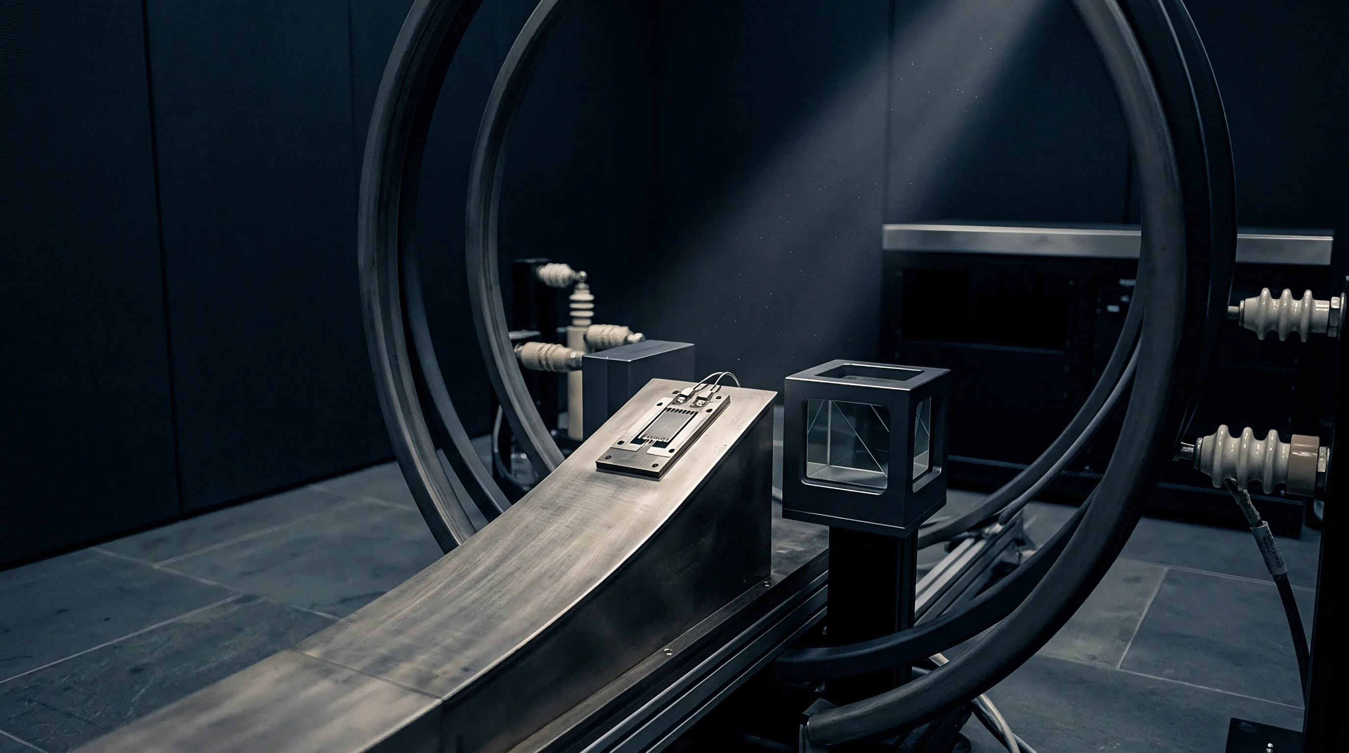
Thermal chamber characterization establishes the limits of factory polynomial compensation. The sensor undergoes soak profiles consisting of discrete thermal plateaus separated by controlled ramp rates. A typical profile sweeps from minus forty degrees Celsius to plus eighty-five degrees Celsius in increments of fifteen degrees, dwelling at each temperature point for three hours to achieve thermal equilibrium across the package core.
Sampling the sensor output during steady-state soak periods isolates intrinsic noise parameters at each distinct operating temperature.
| Modality Type | Thermal Bias Drift | Scale Factor Shift | Allan Variance Floor | Dominant Thermal Mechanism |
|---|---|---|---|---|
| Consumer Capacitive Silicon | 15.0 deg/hr/C | 120 ppm/C | 8.0 deg/hr | Die-attach asymmetry stress |
| Industrial MEMS Silicon | 1.2 deg/hr/C | 35 ppm/C | 0.8 deg/hr | Silicon suspension flexure expansion |
| Tactical Quartz Flexure | 0.08 deg/hr/C | 5 ppm/C | 0.03 deg/hr | Quartz dimensional thermoelasticity |
| Interferometric Fiber Optic | 0.005 deg/hr/C | 0.8 ppm/C | 0.001 deg/hr | Shupe effect coil winding gradients |
The Shupe effect in fiber optic gyroscopes illustrates the extreme consequence of spatial thermal gradients. Non-symmetric time-dependent temperature distributions along the fiber coil generate non-reciprocal optical phase shifts that mimic rotational inputs. In capacitive MEMS devices, asymmetric thermal expansion of the lead-frame generates package warpage, tilting the internal proof mass capacitive sense fingers by sub-nanometer distances.
This microscopic tilt manifests as an apparent milli-g offset shift on an accelerometer channel or a multi-degree-per-hour rate offset on a gyroscope axis.
Quantifying thermal hysteresis requires running matching soak schedules in ascending and descending directions. The resulting Allan variance plots reveal whether structural stress settles elastically or generates irreversible offsets. An improperly cured epoxy die-attach exhibits mechanical relaxation hysteresis, shifting the flicker noise floor upward by an order of magnitude between heating and cooling sequences.
Failure to map the temperature dependence of Allan variance parameters forces downstream system integrators to over-design external sensor fusion filters. When a Kalman filter assumes a static angle random walk coefficient determined only at twenty-five degrees Celsius, the filter diverges rapidly when the vehicle operates across sub-zero cold starts or high-temperature engine compartments.
Conversion
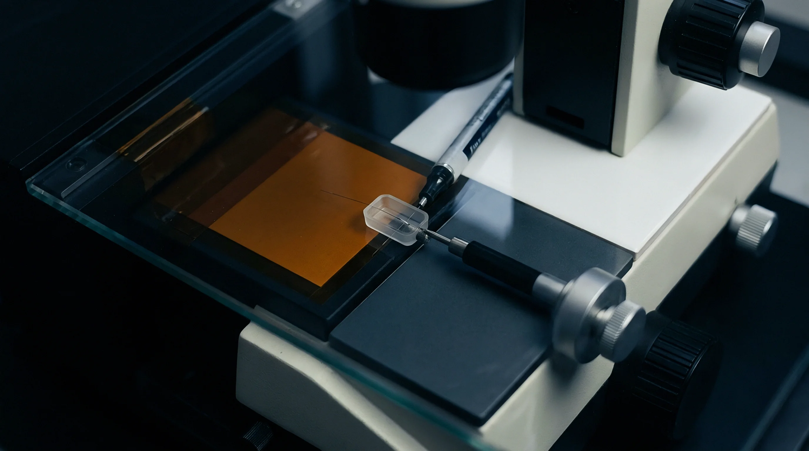
The electronic signal chain that captures the sensor output imposes an absolute hardware noise ceiling on the characterization process. An analog-output inertial sensor requires an external analog-to-digital converter whose quantization noise, effective number of bits, and input voltage noise density sit comfortably below the physical transducer noise floor. If an engineer pairs a tactical-grade MEMS gyroscope having a white noise floor of point zero zero five degrees per second per root hertz with a sixteen-bit SAR converter operating across a wide dynamic range, ADC quantization dominates the short-cluster region of the Allan deviation curve.
The quantization noise parameter Q appears on the Allan deviation plot with a characteristic slope of negative one. The theoretical magnitude follows the relationship where sigma of tau equals the square root of three times Q divided by tau. In digital-output inertial sensors, the internal decimation filter shapes this noise before data reaches the SPI or I2C bus.
Modern sigma-delta converters utilize digital low-pass filtering to clear high-frequency quantization noise outside the operational passband. If this filtering introduces sinc-filter ripple or out-of-band aliasing, the short-tau Allan deviation data distorts, curving downward artificially at the sampling interval limit.
A 24-bit delta-sigma converter with under three microvolts RMS noise is mandatory to resolve sub-micro-g accelerometer flicker floors.
Clock jitter and sampling frequency stability play a decisive role in long-duration Allan variance logs. Over a continuous seventy-two-hour characterization run, drift in the master crystal oscillator alters the effective cluster bin width tau. A timing drift of ten parts per million across hundreds of thousands of samples shifts the bin aggregation edges, leaking low-frequency phase noise into the calculation.
This sampling jitter artificially raises the measured rate random walk coefficient. High-precision characterization benches lock the data acquisition clock to an oven-controlled crystal oscillator or a rubidium atomic standard.
Interpreting digital inertial measurement unit outputs requires inspecting the internal decimation and integration registers. Many integrated six-axis IMUs provide delta-theta and delta-velocity registers rather than raw instantaneous rates. These registers report integrated angular and linear increments accumulated over the internal sample period.
Computing Allan variance directly from delta-theta registers bypasses external numerical integration errors, providing a direct measurement of the intrinsic random walk parameters established by the internal ASIC.
Flaws
Characterizing an inertial sensor by Allan variance introduces subtle systemic traps that invalidate the resulting error coefficients. Practitioners frequently mistake environmental contamination for intrinsic transducer physics. The table below outlines recurring experimental errors, their direct symptoms on the log-log plot, and the procedural interventions needed to correct them.
| Experimental Error | Plot Symptom | Physical Mechanism | Corrective Procedure |
|---|---|---|---|
| Insufficient Record Length | Erratic scatter at large tau values | Low statistical degrees of freedom | Log data for at least 10 times the longest tau of interest |
| Building HVAC Cycling | Sinusoidal hump at tau 15 to 45 min | Diurnal and air-handler thermal cycling | Implement active thermal shielding with vacuum isolation |
| Mains Ground Loop | Elevated white noise floor (slope -0.5) | 50/60 Hz line pickup aliasing into passband | Use isolated battery power and single-point grounding |
| Acoustic Rectification | Unstable bias instability minimum | Sound pressure driving suspension resonance | Enclose sensor in dense acoustic isolation shroud |
| Improper Detrending | False ramp slope (slope +1.0) | Systematic turn-on warm-up drift inclusion | Discard the initial 2 hours of thermal settling data |
A frequent error involves treating the raw experimental data without removing deterministic turn-on thermal transients. Every inertial sensor exhibits a warm-up period during which internal self-heating of the ASIC and proof mass alters mechanical clearances. If this initial transient remains in the dataset, a steep positive slope of plus one dominates the long-cluster regions of the plot, completely burying the true stochastic bias instability minimum.
The characterization sequence must drop the initial ninety to one hundred twenty minutes of data, capturing only the steady-state thermal phase.
Data truncation errors corrupt the opposite end of the spectrum. An engineer logging data for eight hours cannot reliably extract bias instability that occurs at a tau of two hours. At a tau equal to one-quarter of the total logging time, the overlapping Allan variance estimator operates on very few independent data clusters, expanding the ninety-five percent confidence interval bounds until the extracted number becomes an operational gamble.
Reliable parameter extraction demands a continuous recording duration at least ten times longer than the largest tau parameter entered into the navigation filter model.
Selection
Deciding between inertial sensor transduction technologies fixes the achievable Allan variance noise boundaries before a board layout begins. Silicon MEMS dominates volume markets but presents fundamental physical barriers to ultra-low bias drift. The small proof mass of a silicon accelerometer limits mechanical sensitivity, requiring high capacitive pick-off amplification gains that elevate the white noise floor.
In contrast, tactical-grade quartz flexure accelerometers use macroscopic quartz crystal hinges with superior dimensional stability, achieving sub-micro-g bias repeatability at five to ten times the component cost.
In rotational rate sensing, the divide between MEMS Coriolis vibratory elements, optical ring lasers, and fiber optic coils is stark. Coriolis gyroscopes rely on mechanical resonance of tiny silicon rings or tuning forks. Thermal energy dissipation within the silicon lattice establishes a thermo-mechanical noise floor that bounds the angle random walk.
Fiber optic gyroscopes bypass moving mechanical structures entirely, using the Sagnac effect to measure the phase difference between counter-propagating light beams inside a continuous spool of optical fiber. The noise floor in optical instruments is governed by photonic shot noise at short integration intervals and thermal winding gradients at long integration intervals.
- Consumer silicon Coriolis gyroscopes deliver angle random walk between zero point one and zero point five degrees per root-hour, with flicker floors flattening near five to ten degrees per hour, answering short-horizon mobile device gestures.
- Industrial-grade silicon MEMS IMUs yield angle random walk figures near zero point zero three degrees per root-hour and flicker floors under one degree per hour, enabling commercial drone flight control and mobile mapping.
- Tactical closed-loop fiber optic gyroscopes drop angle random walk below zero point zero zero five degrees per root-hour, holding bias stability beneath point zero one degrees per hour for autonomous subsea navigation.
- Navigation-grade ring laser gyroscopes push random walk down to zero point zero zero one degrees per root-hour with bias drift crossing below point zero zero one degrees per hour, supporting commercial aviation inertial reference units.
Procuring tactical-grade performance introduces steep supply-chain realities. Silicon MEMS foundries capable of producing sub-degree-per-hour bias instability devices are concentrated among a limited number of specialized facilities in North America, Europe, and Japan. High-performance quartz flexure sensors and precision optical gyroscopes face strict export controls under the International Traffic in Arms Regulations and dual-use commerce control lists.
Sourcing an instrument with over-specified Allan variance parameters risks severe regulatory friction, extended delivery horizons of twenty-six to forty weeks, and non-recurring engineering charges for custom calibration fixture tooling.
The contract documentation for high-reliability sensor procurement must explicitly cite the testing protocols used to validate Allan variance claims. Standard purchase specifications should mandate that the vendor supply raw time-series data for each delivered batch, accompanied by calibration dossiers confirming that the sensor bias instability was measured on an isolated seismic foundation conforming to IEEE Std 952 Annex C.