Piezoresistive Pressure Sensor Signal Conditioning Conditioning Polynomial Calibration Chamber Testing
Normalizing digitized bridge and temperature counts before solving polynomial matrix equations eliminates floating point overflow and preserves calibration accuracy.

Die
Microelectromechanical piezoresistive pressure sensing elements rely on longitudinal and transverse piezoresistive effects within a micromachined monocrystalline silicon diaphragm. P-type piezoresistors, diffused or ion-implanted along specific crystallographic directions, convert diaphragm flexure into fractional resistance changes. Fluid pressure deflects the thin diaphragm, creating tensile stress in piezoresistors parallel to the diaphragm edges and compressive stress in those set perpendicular to the edges.
This layout yields two resistor pairs with resistance shifts of equal magnitude but opposite signs.
Diaphragm stress directly drives signal gain. Wiring these four active elements into a fully differential Wheatstone bridge maximizes full-scale output voltage and suppresses common-mode noise. Silicon strain elements are more than an order of magnitude more sensitive than conventional metal foil gauges: standard gauge factors for P-type silicon piezistors range between 100 and 170, compared to roughly 2.0 for metallic foil.
That sensitivity produces full-scale spans from 20 mV/V to 200 mV/V under nominal bridge excitation voltages, keeping raw millivolt signals well above the noise floor of precision instrumentation circuits.
A p-type silicon piezoresistor array on a 100 crystallographic plane exhibits a negative temperature coefficient of sensitivity reaching minus 0.22 percent per degree Celsius under constant voltage excitation across the minus 40 to 125 degree Celsius operating band.
Uncompensated raw silicon elements suffer severe measurement distortion from thermal drift. Two primary temperature coefficients dictate this behavior: the Temperature Coefficient of Resistance, tracking baseline bridge impedance over temperature, and the Temperature Coefficient of Sensitivity, measuring the decay of piezoresistive coefficients as thermal energy increases in the silicon lattice. Piezoresistance drops at higher temperatures because carrier scattering degrades mobility in the doped conduction channels.
Under constant voltage drive, full-scale output span contracts at rates typically between minus 0.15 percent per degree Celsius and minus 0.30 percent per degree Celsius. Zero-pressure offset voltage also drifts unpredictably, driven by thermal expansion mismatches between the silicon die, the glass frit or eutectic die-attach layer, and the supporting ceramic or metal header assembly.
Deflection mechanics introduce non-linearities into the transfer curve. At low deflection ratios, where diaphragm thickness is several times greater than center displacement, small-deflection plate theory applies and output remains nearly linear. Once applied pressure pushes center displacement past 20 percent of diaphragm thickness, large-deflection membrane stresses develop, stiffening the structure non-linearly.
This compresses the output span at higher pressures, leaving baseline non-linearity figures typically between 0.1 percent and 0.5 percent of full scale span. Packaging adds further complexity: protective gel encapsulation for liquid isolation imparts shear stress across the diaphragm face, shifting the zero-pressure offset and introducing thermal hysteresis during rapid temperature shifts.
These inherent physical error sources in raw micromachined piezoresistive elements must be classified before designing the signal conditioning stage.
- Piezoresistive Strain Saturation limits maximum linear output voltage at high pressures due to carrier mobility limits in heavily doped P-type silicon channels.
- Thermal Expansion Mismatch Drift shifts zero-pressure bridge offset voltage via residual mechanical stress across the interfaces of silicon, glass, and metal assemblies.
- Silicone Gel Shear Coupling transfers mechanical forces across the diaphragm surface as temperature shifts expand or contract protective gel compounds.
- Diaphragm Edge Stress Concentration drives non-linear resistance changes as pressure forces approach the mechanical yield strength of the micromachined silicon boundary walls.
Baseline offset shifts occurring after solder reflow reflect normal package stress relaxation rather than manufacturing defects.


Amplification
Front-end analog processing transforms low-level differential bridge signals into digitized readings for host processing. Excitation architecture directly affects thermal stability. Constant voltage drive is simple, but it leaves the signal chain exposed to the negative temperature coefficient of piezoresistive sensitivity.
Constant current excitation, on the other hand, provides passive first-order thermal compensation. Because silicon bridge resistance increases with temperature according to its positive temperature coefficient of resistance, driving a fixed current through the bridge forces a compensating rise in bridge supply voltage. This rising excitation voltage offsets decaying strain sensitivity, cutting raw thermal span drift by up to 80 percent without firmware intervention.
Modern digital sensor signal conditioner ICs combine programmable gain instrumentation amplifiers with high-resolution ADCs to process bridge signals. Chopped input topologies eliminate low-frequency 1/f noise and front-end offset drift, keeping input-referred noise densities below 25 nV per square-root Hertz. Programmable gain stages match the full-scale span of the sensor die to the converter’s dynamic input range.
With gain settings scaling from 1 to 256, a single ASIC can handle sensor dies with broad sensitivity variations, standardizing downstream hardware across multiple pressure ranges.

Signal Conditioner Front End Architecture Comparison
| Architecture Type | Excitation Mechanism | TCS Self Compensation | Dynamic Range (mV/V) | Supply Rejection Ratio (dB) | Typical System Cost (USD) |
|---|---|---|---|---|---|
| Discrete Op-Amp Network | Constant Voltage | None | 10 to 50 | 65 | 1.10 |
| Passive Thermistor Compensated | Constant Current | First Order Partial | 15 to 60 | 72 | 1.85 |
| Integrated Programmable ASIC | Ratiometric Current/Voltage | Active Digital Compensation | 1 to 256 Range | 95 | 3.40 |
| Direct Delta-Sigma Digitizer | Ratiometric Voltage Drive | Digital Polynomial Matrix | 2 to 128 Range | 105 | 2.90 |
The choice of ADC architecture determines overall measurement resolution and noise immunity. Delta-sigma converters dominate here because of their high oversampling ratios and natural low-pass noise shaping. Effective resolution depends heavily on signal bandwidth and output sample rate: a 24-bit delta-sigma converter running at a 10 Hz conversion rate reaches an effective number of bits exceeding 19.5 bits ~ a peak-to-peak noise floor below 1 part in 500,000 of full scale span.
Pushing the sample rate to 1 kHz shifts the noise corner higher, dropping effective resolution to 16.2 bits.
Meeting IEC 61326 clause 6.2 requires signal line decoupling that limits RF input-rectified offset shifts to under 0.05 percent of full scale span in a 10 volt per meter field.
Ratiometric design eliminates errors from power supply drift. When the ADC reference voltage comes directly from the supply rail powering the piezoresistive bridge, supply fluctuations scale both the bridge output and the ADC reference proportionally. Because the digital output code represents the ratio of bridge voltage to reference voltage, digitized measurements become immune to supply rail variations.
Overall accuracy then depends on internal amplifier drift, passive component tolerances, and converter linearity rather than external regulator performance.
An unshielded current trace coupling 45 microvolts of power supply ripple into the instrumentation front end ruined twelve fully encapsulated prototype manifolds.
Polynomial
Mathematical error correction models eliminate residual physical non-linearities and thermal cross-sensitivities by running raw bridge and temperature values through surface-fitting algorithms. Conditioning ASICs run multi-variable polynomial matrices to extract calibrated pressure readings from non-linear analog inputs. The ADC returns a unitless count representing mechanical strain, while an internal diode array or thermistor provides a simultaneous count for junction temperature.
The engine then evaluates a two-dimensional surface polynomial using both inputs to calculate pressure.
Which Polynomial Term Order Prevents Matrix Ill Conditioning?
Selecting the optimal polynomial order means balancing residual fit error against calculation complexity and numerical stability. A standard bivariate polynomial expands as follows:
P(S, T) = a00 + a10 S + a01 T + a20 S^2 + a11 S T + a02 T^2 + a30 S^3 + a21 (S^2) T + a12 S (T^2) + a03 T^3
Here, P is calculated pressure, S is normalized bridge signal counts, T is normalized temperature counts, and coefficients a_ij are calibration factors stored in non-volatile memory. Third-order terms in S compensate for diaphragm deflection non-linearities, while second-order terms in T correct non-linear temperature coefficients of resistance and sensitivity. Cross-terms like S T capture the temperature dependence of piezoresistive span.
Matrix ill-conditioning is a primary failure mode when deriving polynomial coefficients. Feeding unscaled 24-bit converter counts (from 0 to 16,777,215) into high-order terms like S^3 expands the dynamic range toward 4.7 x 10^21. Running matrix inversion on values spanning such extreme magnitudes causes severe floating-point truncation and catastrophic cancellation during least-squares regression.
Normalizing raw signal and temperature counts into a centered interval between -1.0 and +1.0 before running matrix calculations avoids this issue.
Normalizing sensor bridge raw counts to a centered domain prior to coefficient matrix inversion prevents catastrophic floating point cancellation during higher order surface fitting.
Least-squares surface regression solves the over-determined system of equations built during calibration. Gathering data across M discrete temperature points and N pressure points produces an M x N grid. Solving the normal equations (A^T A) X = A^T B yields coefficient matrix X, which minimizes residual pressure error across the operating envelope.
Embedded microcontrollers lacking floating-point units evaluate these polynomials using scaled fixed-point integer arithmetic, which requires careful bit-shift allocation during intermediate multiplications to prevent register overflow without sacrificing lower-bit precision.

Polynomial Evaluation Accuracy across Grid Sizes
| Polynomial Order (S x T) | Total Matrix Coefficients | Minimum Calibration Grid | Max Fit Residual (% FS) | Fixed Point Compute Time (μs) | Memory Footprint (Bytes) |
|---|---|---|---|---|---|
| 1st Order (1 x 1) | 4 Coefficients | 2 Temp x 2 Press | 0.850 | 12 | 16 |
| 2nd Order (2 x 2) | 9 Coefficients | 3 Temp x 3 Press | 0.085 | 38 | 36 |
| 3rd Order Signal (3 x 2) | 12 Coefficients | 3 Temp x 4 Press | 0.015 | 64 | 48 |
| Full 3rd Order (3 x 3) | 16 Coefficients | 4 Temp x 4 Press | 0.008 | 110 | 64 |
Quantization noise in the temperature channel directly creates uncertainty in the calculated pressure. Because temperature cross-terms scale pressure corrections, noise on the temperature path turns into synthetic pressure jitter. High-precision conditioners apply low-pass digital filtering to the temperature ADC channel, keeping temperature noise below 0.02 degrees Celsius RMS.
With a 12-coefficient matrix, residual fitting errors stay under 0.02 percent of full scale span across a -40 to +125 degree Celsius operating band.
Whether dynamic non-linear thermal hysteresis in gel-filled stainless steel housings can be mapped by static polynomial matrices without introducing high-order polynomial oscillation between calibration points remains an open question.
Heat
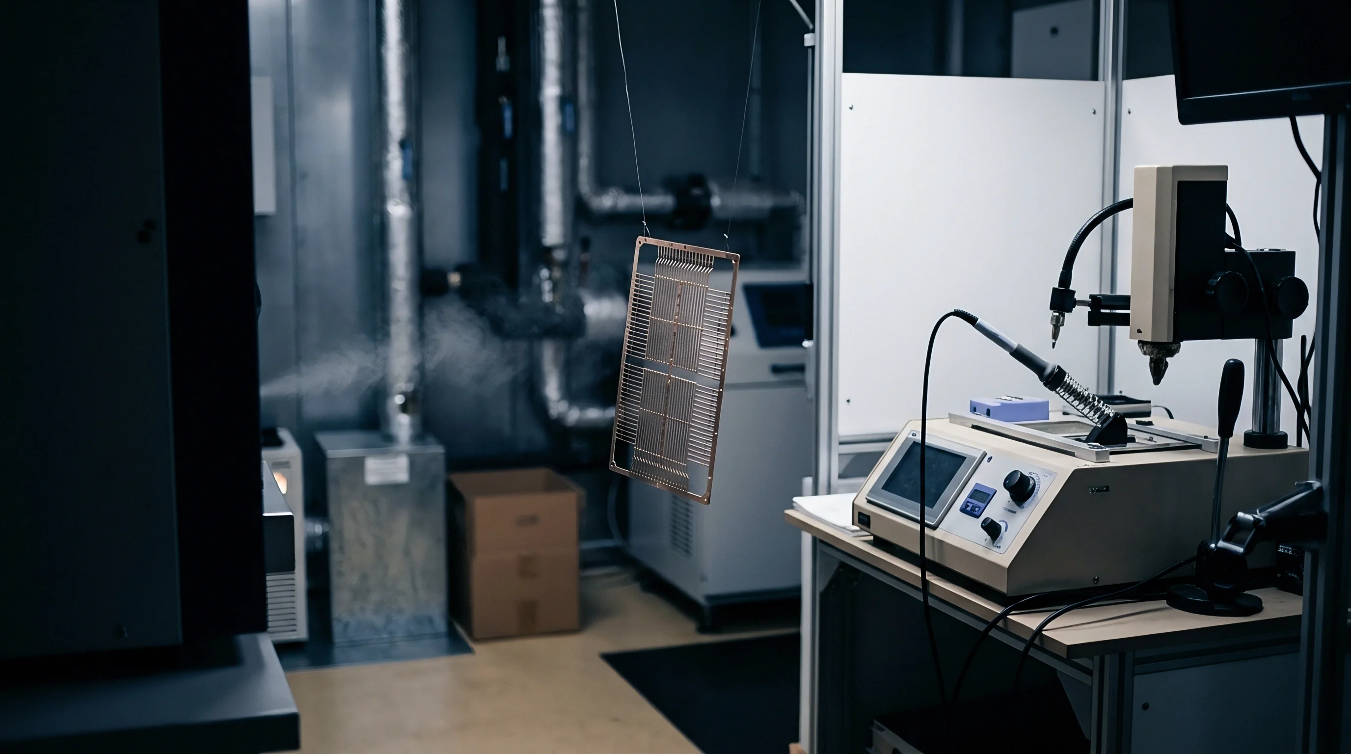
Environmental chamber runs establish the boundary conditions needed for valid calibration datasets. Thermal equilibrium across the test volume determines data integrity. Inside the chamber, sensors undergo radiative heat exchange with chamber walls, convective exchange with moving air, and conductive transfer through wiring and pressure plumbing.
Packaged silicon dies in heavy metal housings or oil filled cavities have significant thermal time constants; chamber air stabilizes long before internal die temperatures reach equilibrium.
Transient thermal gradients across a sensor invalidate calibration points. During rapid temperature shifts, the outer metal housing expands or contracts faster than the internal ceramic substrate, inducing mechanical bending stresses that reach the silicon diaphragm. These transient strains produce large, non-repeatable offset spikes that mask steady-state behavior.
Calibration protocols therefore rely on controlled ramp rates and extended dwell times to guarantee complete thermal stabilization before taking readings.
- Set environmental chamber temperature ramp rate to a maximum of 1.5 degrees Celsius per minute to limit thermal stress gradients across the package housing.
- Hold chamber temperature at the soak setpoint for at least 45 minutes to allow complete thermal equilibration of the internal ceramic substrate mass.
- Apply pressure calibration increments from zero to full scale in 20 percent span steps using high-purity nitrogen gas.
- Allow a 30-second dwell at each pressure step for gas adiabatic thermal dissipation before logging raw bridge ADC and temperature sensor counts.
- Repeat the pressure stepping sequence in descending order down to zero pressure to quantify mechanical diaphragm hysteresis.
Gas thermodynamics inside pressure supply lines introduce thermal artifacts during rapid pressure steps. Pressurizing a closed manifold causes adiabatic compression, heating gas locally inside the sensor cavity. Venting gas during step-down cycles has the opposite effect, causing expansion cooling.
Reading sensor outputs immediately after a step captures these thermal transients and distorts non-linearity measurements. Calibration software must use stabilization timers to delay data logging until gas pressure and temperature fully settle.
Calibration dwell times at temperature setpoints should always exceed the thermal relaxation time of the heaviest metal mass in the test fixture.


Rig
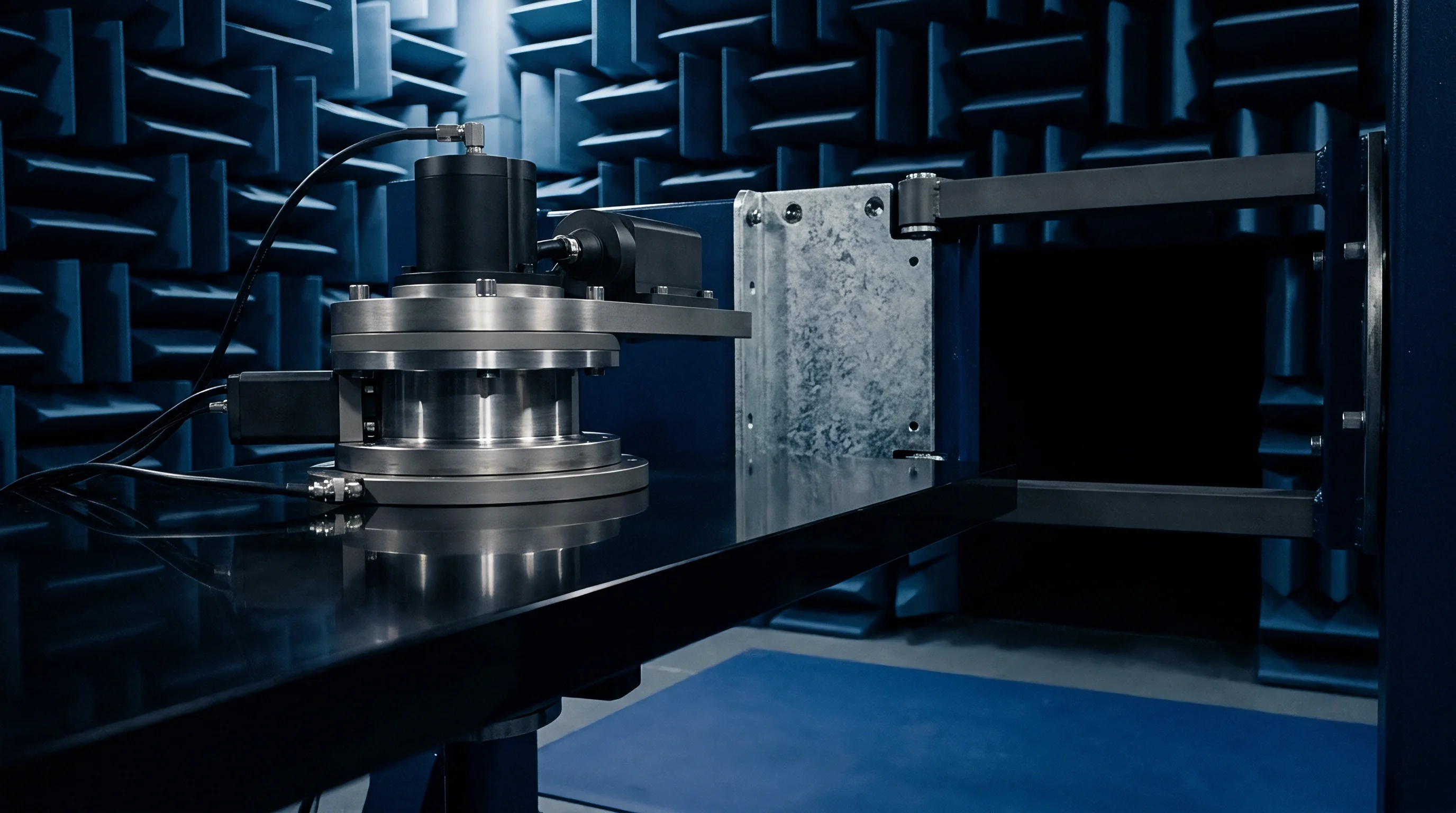
Automated calibration equipment must synchronize environmental profiling, pressure delivery, signal acquisition, and coefficient programming across large sensor batches. Pressure controllers use dual-piston quartz reference transducers to deliver target pressures with expanded measurement uncertainties below 0.01 percent of reading. Digital interfaces link the primary pressure controller, chamber controller, data acquisition scanners, and device programmers into a single control loop.
Automated calibration workflow follows a deterministic sequence designed to maximize throughput while preserving measurement accuracy.
- Thermal Chamber Soak Synchronization establishes verified isothermal conditions across all device-under-test positions before pressure stepping begins.
- Primary Pressure Reference Stabilization commands the pneumatic controller to target pressure setpoints and monitors stability until pressure noise drops below 0.002 percent span.
- Synchronous Data Logging Capture triggers simultaneous acquisition of raw digital signal and temperature counts across all multiplexed device channels over dedicated parallel buses.
- Least Squares Matrix Regression Execution transmits pooled raw dataset blocks to host software to solve the over-determined polynomial matrix equations.
- ASIC Non-Volatile Memory Flashing writes calculated multi-variable correction coefficients directly into device EEPROM registers via one-wire or I2C protocols.
- Independent Verification Audit Pass runs a secondary pressure and temperature sequence at intermediate points to verify post-calibration accuracy against pass-fail limits.
Multiplexing microvolt-level analog bridge signals introduces parasitic thermal electromotive forces across relay contacts and connector pins. Dissimilar metal junctions under subtle thermal gradients generate Seebeck voltages up to several microvolts per degree Celsius, corrupting zero-pressure offset measurements. High-density calibration fixtures mitigate thermal EMF by using solid-state, low-leakage analog multiplexers or by digitizing signals at each sensor socket with local ASICs before routing data digitally.
Automated Calibration Test Rig Throughput Comparison
| Fixture Architecture | Batch Capacity (Units) | Multiplexing Modality | Cycle Time per Batch (Hours) | Expanded Calibration Uncertainty | Capital Equipment Cost (USD) |
|---|---|---|---|---|---|
| Central Analog Scanner | 64 | Low EMF Reed Relay | 8.5 | 0.05% FS | 45,000 |
| Parallel Digital Socket Array | 128 | Direct SPI/I2C Bus | 5.2 | 0.02% FS | 82,000 |
| Fully Automated Matrix Cell | 256 | Isolated CANbus Array | 3.8 | 0.01% FS | 165,000 |
Verification testing checks calibration algorithm performance against independent criteria. Once coefficients are programmed into ASIC non-volatile memory, the rig runs the batch through a verification profile using test points located midway between the original calibration grid points. This step catches Runge phenomena, where higher-order fitted curves oscillate unnaturally between calibration points.
Batches showing residual verification errors above target limits are flagged for automatic rejection and triage.
Under ISO 17025 section 7.7, verification requires that reference pressure standard uncertainty maintain an expanded uncertainty ratio of at least four to one relative to the sensor target specification.

Procurement
Sourcing piezoresistive pressure sensors involves balancing component integration, calibration overhead, and supply chain complexity. Buying uncompensated bare MEMS dies keeps initial BOM costs down, but shifts substantial technical burden and capital expenditure to manufacturing. End-of-line factory calibration demands high-density thermal chambers, precision pressure controllers, custom fixtures, and long cycle times.
In practice, calibration machine-hour costs frequently exceed the purchase price of the bare silicon die.
Commercial procurement choices fall into three main architectural models: bare MEMS die paired with discrete analog signal chains, bare die integrated with custom digital ASICs, or fully calibrated OEM sensor modules. The choice determines both up-front capital investment and long-term unit cost scaling.
Commercial Integration Model Cost Analysis
| Integration Strategy | Raw Component BOM Cost (USD) | Calibration Chamber Time (s) | In-House Testing Cost (USD) | Landed Unit Cost (USD) | Supply Chain Exposure Risk |
|---|---|---|---|---|---|
| Bare Die + Discrete Conditioning | 1.20 | 420 | 3.80 | 5.00 | High Process Risk |
| Bare Die + Integrated ASIC | 2.80 | 180 | 1.60 | 4.40 | Moderate ASIC Single Source |
| Pre-Calibrated OEM Module | 6.50 | 0 | 0.15 | 6.65 | Low In-House Capital Exposure |
Wafer-level sensitivity variation complicates yield management in high-volume production. Standard MEMS fabrication yields sensitivity variations up to ±15 percent across a single 8-inch silicon wafer, with baseline offset distributions reaching ±20 mV/V. Signal conditioning ASICs need enough gain adjustment range and offset trim DAC resolution to absorb these variations without sacrificing digital signal resolution. Wafer-level sensitivity variations require strict incoming acceptance thresholds during lot qualification audits to protect assembly line yield.
Selecting a strategic supplier requires evaluating key technical criteria across prospective vendors:
- Wafer Level Sensitivity Distribution Audit verifies that element output span variations fall within the programmable gain window of target signal conditioning chips.
- Signal Conditioning ASIC Protocol Lock Evaluation flags proprietary EEPROM interfaces that could block future drop-in replacements from alternate silicon vendors.
- Calibration Chamber Machine Hour Allocation models factory-floor capital requirements to balance in-house volume scaling against purchasing pre-calibrated OEM modules.
- Second Source Package Drop-In Compatibility checks mechanical, dimensional, and pinout equivalency across alternate foundry suppliers to eliminate single-source risks.
Offloading polynomial coefficient calculation to factory end of line testing transfers thermal chamber capital expense directly onto component unit price.
Automotive and industrial quality standards mandate rigorous qualification for piezoresistive sensing assemblies. Meeting AEC-Q103 requirements demands high-temperature operating life testing, severe thermal shock, and mechanical vibration qualification. Audits should verify that foundries and packaging facilities maintain statistical process controls on die-attach glue thickness, bond wire pull strength, and gel pot consistency.
Fluctuation in these packaging variables degrades long-term calibration stability, causing baseline offset drift in the field.
Dual-sourcing strategies require clear drop-in mechanical and electrical specifications across vendors. Piezoresistive dies from different foundries feature distinct piezoresistive coefficients, bridge impedances, and temperature coefficients. While signal conditioning ASICs absorb these differences during calibration by recalculating polynomial coefficients, physical housing dimensions, port geometries, and gel formulations must remain strictly standardized.
Maintaining structural interchangeability ensures manufacturing lines can swap silicon suppliers without redesigning calibration rigs or altering host firmware.