Thermal Hysteresis and the Settling Time Nobody Budgets
Unbudgeted sensor thermal settling times and hysteresis generate severe measurement errors, demanding mandatory package-level soak protocols to preserve field accuracy.

Mass

Thermal Mass Dynamics and Non-Isothermal Drift
Precision sensing elements sit inside housing engineered for mechanical protection, electrical isolation, and environmental sealing. That internal thermal mass builds in a delay between ambient temperature swings and the true equilibrium of sensitive junctions. Sensor datasheets often publish electrical response times ~ like a ninety percent step response measured in milliseconds inside an agitated liquid bath.
But field installations deal with thermal conduction through mounting brackets, radiation from nearby power components, and convective resistance in stagnant air pockets. As a result, the package’s internal micro-environment can lag behind external fluid temperatures anywhere from tens of seconds to multiple hours.
Thermal gradients across dissimilar materials cause internal mechanical strain via differential thermal expansion. Silicon substrate sensors, strain gauge bridges, and quartz resonant elements turn this structural stress into parasitic electrical signals. When an assembly undergoes a sudden temperature shift from twenty degrees Celsius to eighty degrees Celsius, the outer housing expands right away while the internal substrate stays cool.
Shear stress then spreads across epoxy interfaces, glass seals, and wire bond pads, producing offset drift that stems from mechanical distortion rather than actual ambient temperature changes.
| Enclosure Material | Internal Volume (cm³) | Convective Resistance (K/W) | Thermal Time Constant (s) | Ninety-Nine Percent Settling Time (min) |
|---|---|---|---|---|
| Anodized Aluminum 6061 | 45 | 4.2 | 120 | 9.2 |
| Stainless Steel 316L | 45 | 11.8 | 340 | 26.1 |
| Polycarbonate PBT Compound | 45 | 28.5 | 810 | 62.1 |
| Hermetic Titanium Grade 5 | 22 | 14.1 | 290 | 22.2 |
Heat dissipation along sensor wiring acts as a secondary conduction path during thermal transients. Copper leads carry heat to internal sensing elements much faster than plastic housing walls dissipate energy into surrounding air. This path can create internal temperature differences up to three degrees Celsius during active heating.
Until the entire assembly reaches thermal equilibrium, sensor output reflects this internal imbalance. Estimating settling times based only on the sensing element’s thermal mass routinely overlooks these package-level conduction channels.
Standard test protocols operating under liquid immersion understate field settling times in still air by a factor of eight.
Active excitation introduces self-heating into the thermal balance. A resistance temperature detector driven at two milliamperes dissipates power directly within its ceramic core, creating an internal offset that varies with external dissipation conditions. In stagnant air, self-heating raises the core temperature above the fluid temperature by fractions of a kelvin.
If fluid velocity changes, the heat transfer coefficient shifts as well, altering the self-heating equilibrium and registering as a false temperature change. Telling fluid temperature variations apart from self-heating shifts requires longer observation windows.
Material interfaces inside the sensor undergo micro-structural relaxation long after bulk thermal equilibrium seems complete. Polymer potting compounds exhibit viscoelastic creep under thermal strain, releasing stored mechanical stress slowly over time. This gradual strain relief shifts the pressure on sensitive silicon dies, driving output drift long after external thermocouples register a stable housing temperature.
Bench verification has to run well past initial temperature stabilization to catch these long relaxation tails.
Settling time models often rely on single-exponential decay assumptions derived from lumped capacitance approximations. Real sensor packages, however, contain distinct thermal masses linked by finite conductivities. Their actual step response is a sum of multiple exponential terms with widely varying time constants.
Automated test software is easily tricked by a fast initial decay phase, declaring stability while long-term slow terms remain unmeasured.
Mechanical Strain Recovery in Encapsulated Substrates
Encapsulated sensors undergo micro-scale mechanical displacements during thermal cycling. Die-attach adhesives, solder joints, and conformal coatings expand at different rates, and these CTE mismatches store elastic energy inside the housing as temperatures rise. When the package cools back to baseline, the internal stress field does not trace the original path back down.
Instead, mechanical strain hysteresis leaves residual stress that shifts both sensor sensitivity and zero-point offset.
Silicon piezoresistive pressure transducers are particularly sensitive to package strain hysteresis. The die bond interface deforms elastically during excursions up to eighty-five degrees Celsius. Cooling back to twenty-five degrees Celsius causes microscopic slip along epoxy filler interfaces, leaving residual shear across the silicon diaphragm.
The bridge output then shows an offset error proportional to how high the temperature swung. Without sufficient settling time, these residual stresses never relax back to baseline.
Cycling through a twenty to eighty degree temperature cycle produces residual baseline shifts that can require seventy-two hours of unpowered room-temperature soak to decay within published specifications.
Structural relaxation inside glass-to-metal hermetic seals follows a power-law time dependence rather than linear decay. Under residual stress from the outer metal sleeve, glass matrices slowly rearrange at the atomic level. This internal strain field can take days to relax, altering feedthrough capacitance and mechanical stress on the sensing element.
Calibration performed within four hours of thermal processing catches a transient strain state, generating coefficients that drift as the material settles over the following weeks.
High-precision strain gauge assemblies face similar mechanical lag inside their adhesive bonding layers. Phenolic and epoxy adhesives absorb moisture and age physically under elevated temperatures. Thermal cycles speed up moisture desorption from the matrix, changing its shear modulus and dimensional stability.
The bonded gauge reads this dimensional change as a false strain signal, and stability returns only after internal moisture equilibrates with ambient humidity.
Polymer housings worsen mechanical strain recovery through creep and physical aging. Thermoplastics such as polyether ether ketone or polyphenylene sulfide contract slowly after exposure to temperatures near their glass transition points. That volumetric shrinkage exerts steady pressure on internal sensing capsules.
QA protocols need thermal pre-conditioning cycles to accelerate post-molding physical aging before calibration begins.
Zero-point offset drift stems directly from this mechanical relaxation lag. In environments with rapid temperature swings, precision instruments suffer steady calibration degradation, trailing true values by an offset dictated by material relaxation time constants. Planning adequate soak times into operational procedures is essential to manage structural hysteresis in the field.

Gradient

Transient Spatial Gradients within Sensor Bodies
Spatial thermal gradients develop across sensor bodies during environmental temperature shifts. Heat flows from external surfaces inward along paths governed by thermal impedance networks. On a heavy industrial probe, the front face encounters ambient changes minutes before the rear connector assembly.
This spatial temperature difference generates thermoelectric voltages, mechanical bowing, and localized resistance shifts across internal bridge circuits. Signals fluctuate during transient heating, stabilizing only after internal spatial gradients fall below critical levels.
Thermoelectric errors crop up when spatial gradients span junctions of dissimilar metals inside sensor wiring. Internal terminal blocks, solder joints, and PCB traces produce parasitic Seebeck voltages during thermal transients. A five degree Celsius gradient across an internal copper-constantan junction pair can generate a parasitic voltage shift over two hundred microvolts.
In low-level signal conditioning, this thermal EMF appears as zero-point offset error until spatial uniformity is restored.
- Thermal Excitation Phase ~ Rapid ambient temperature changes establish steep gradients across housing walls and internal mounting structures.
- Parasitic Signal Generation ~ Thermoelectric junctions and differential strain produce peak electrical errors in signal conditioning pathways.
- Internal Heat Redistribution ~ Conduction within internal components reduces spatial temperature differences while package temperature stabilizes.
- Micro-Structural Relaxation ~ Polymer coatings and mechanical bonds release stored thermal strain along non-linear relaxation curves.
- Asymmetric Equilibrium Attainment ~ Final electrical output settles into an offset dictated by historical thermal directional pathways.
Differential thermal expansion across printed circuit boards causes mechanical flexing during rapid temperature ramps. Surface-mount ceramic capacitors and resistor networks absorb stress transmitted through solder joints, changing passive component values through piezo-resistive and piezo-electric effects. Precision op-amps experience input offset shifts under mechanical stress as well.
The net circuit output reflects these combined physical distortions until the board reaches spatial thermal equilibrium.
ISO/IEC 17025 laboratory audits require documented thermal equilibrium limits prior to executing official calibration protocols.
Sensor designs attempt to minimize spatial gradients using internal copper planes and symmetrical layouts. High-conductivity paths route heat evenly around sensitive measurement cores, while passive thermal shielding delays external heat penetration to soften environmental spikes into gentler ramps. Even so, asymmetric mounting geometries in real installations break thermal symmetry, reintroducing transient spatial gradients that degrade signal integrity.
Field installations frequently expose sensor housings to single-sided thermal loads. Solar radiation heating one side of a flow meter creates a permanent lateral gradient across internal sensing tubes. The resulting structural asymmetry causes zero-flow drift that evades standard zero-point calibrations performed in uniform temperature baths.
Correcting for this requires external thermal insulation or active multi-sensor compensation arrays.
Transient thermal gradients undermine multi-point electronic compensation algorithms in smart sensors. Modern digital units rely on internal temperature sensors to calculate real-time corrections for non-linearity and offset shift. But the compensation sensor sits away from the primary sensing element.
During rapid temperature changes, it reads a different temperature than the core, causing the microprocessor to apply incorrect calibration adjustments. The resulting output error can end up worse than the uncompensated raw sensor drift until spatial equilibrium returns.

Thermal Hysteresis Loops and Path Dependence
Thermal hysteresis occurs when a sensor’s output depends not just on current temperature, but on its preceding thermal history. A sensor evaluated at twenty-five degrees Celsius after cooling from eighty degrees Celsius produces a different signal than the same sensor evaluated at twenty-five degrees Celsius after warming from minus forty degrees Celsius. This gap between ascending and descending calibration curves represents a fundamental limit on measurement accuracy that single-point offset adjustments cannot fix.
Phase transformations and secondary relaxation in sensor materials drive path-dependent output shifts. Magnetoresistive field sensors display thermal hysteresis because domain wall pinning changes during thermal cycles. Piezoelectric ceramic elements undergo domain realignments at elevated temperatures, altering charge coefficients when returned to baseline.
Standard calibration certificates usually document accuracy recorded along a single temperature direction, masking the hysteresis envelope present in real field operations.
Thermal soak outlasts electrical settling time across industrial sensor installations through several distinct physical mechanisms.
Electrical settling happens as decoupling capacitors charge and amplifier bias currents stabilize, usually completing within milliseconds of power-up. Thermal soak, by contrast, involves mass heat transport and mechanical strain relaxation across heterogeneous materials, often taking hours to reach equilibrium. Technicians routinely mistake electrical stability on an oscilloscope for total measurement stability, logging calibration data while internal strain fields are still evolving.
This captures transient figures and injects quiet systematic errors into precision measurement databases.
| Sensor Sensing Technology | Temperature Range (°C) | Hysteresis (% Full Scale) | Dominant Physical Cause | Stabilization Soak Time (Hours) |
|---|---|---|---|---|
| Piezoresistive Silicon Pressure | -40 to +85 | 0.18 | Die-attach polymer strain relaxation | 4.0 |
| Thin-Film Platinum RTD (Class A) | -50 to +200 | 0.04 | Substrate expansion mismatch stress | 1.5 |
| Capacitive Polymer Humidity | +10 to +60 | 1.20 | Water molecule sorption hysteresis | 12.0 |
| Quartz Crystal Microbalance | -20 to +70 | 0.08 | Electrode mounting stress release | 6.0 |
Quantifying thermal hysteresis requires symmetrical closed-loop thermal testing protocols. Testing starts at baseline temperature, ascends to maximum operating limits, soaks until mechanical relaxation is complete, drops to minimum limits, soaks again, and returns to baseline. The maximum output difference recorded at identical intermediate temperature points defines hysteresis magnitude.
Skipping extended soak steps at cycle extremes artificially collapses the measured loop, masking potential field failures.
Sensors deployed outdoors traverse complex daily thermal loops. Solar heating creates top-down thermal paths, while overnight radiative cooling reverses the direction of heat transport. Accumulated hysteresis causes baseline drift over multi-day observation windows.
Calibration performed in the morning yields invalid compensation parameters by the afternoon, forcing procurement teams to specify lower-hysteresis components for critical outdoor use.
High-precision applications require mathematical models of historical thermal paths to compensate for physical hysteresis. Preisach and Prandtl-Ishlinskii models track thermal history to predict signal corrections. Implementing these algorithmic models demands continuous temperature logging, extra microcontroller processing power, and extensive characterization testing for individual sensor lots.
Sourcing teams balancing landed component costs often find that buying lower-hysteresis hardware is cheaper than maintaining custom firmware algorithms.

Relaxation
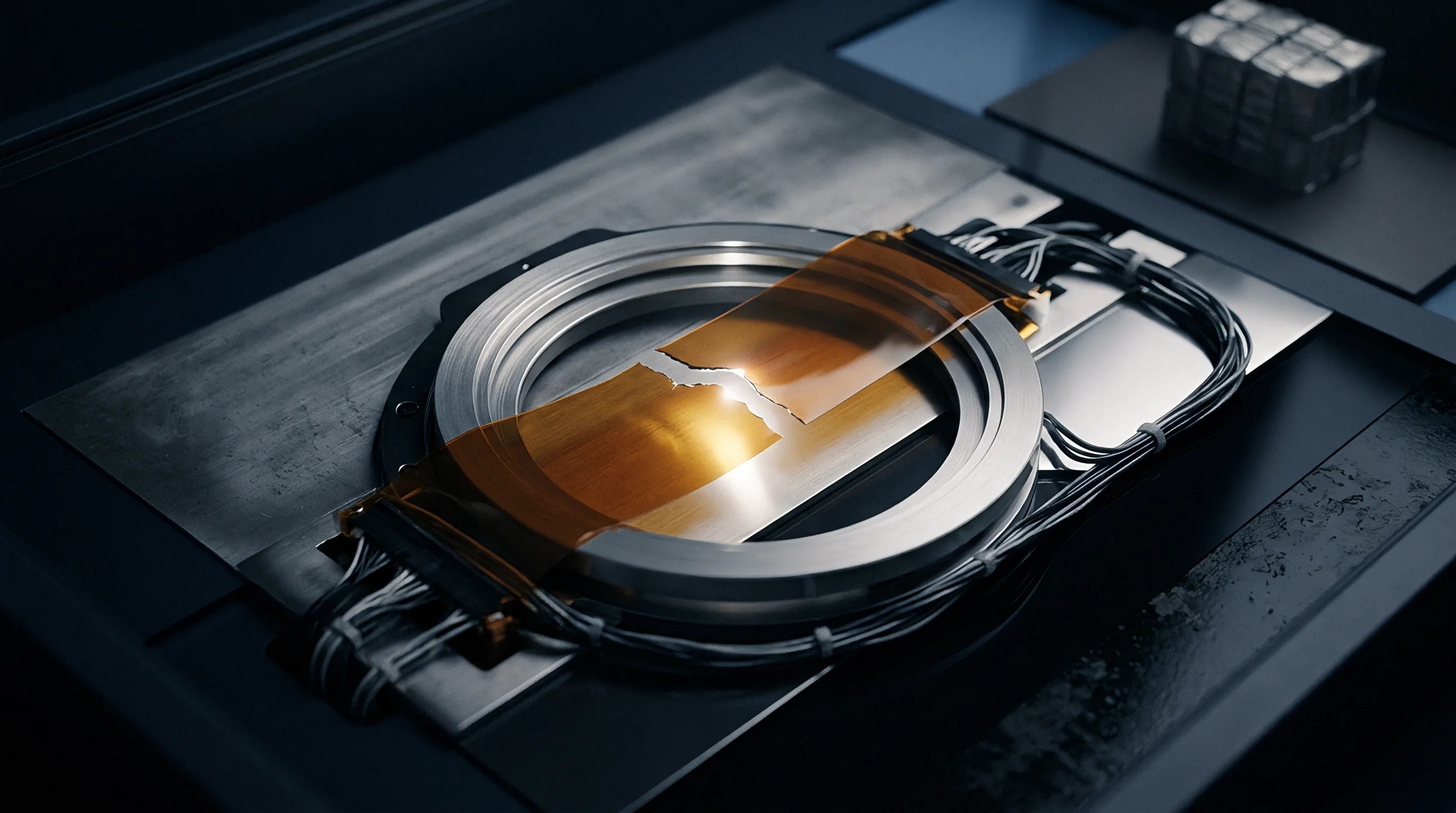
Laboratory Calibration Protocols versus Field Settling Realities
Accredited calibration laboratories operate under tightly controlled environmental limits mandated by standards such as ISO/IEC 17025. Ambient temperature stays locked at twenty degrees Celsius within half a degree, relative humidity remains below fifty percent, and fluid baths provide thermal stability measured in millikelvins. Extended soak periods ensure sensors reach complete thermal and mechanical equilibrium before reference measurements are taken.
Datasheet tolerance claims reflect these ideal conditions ~ representing best-case physical limits rather than expected field performance.
Field installations present real-world challenges that break laboratory assumptions. Ambient temperatures cycle, air currents shift, and mounting structures inject vibration and thermal loads. Taking a sensor from a transit crate at five degrees Celsius and installing it directly into a operating process line at sixty degrees Celsius induces severe thermal shock.
Technicians frequently trim zero points within minutes of installation, confusing initial electrical response with complete package stability. This bakes transient thermal strain directly into the baseline calibration, guaranteeing ongoing measurement error.
- Unconditioned Transit Storage ~ Components held in unconditioned hubs absorb extreme thermal histories that alter material relaxation states.
- Premature Zero-Point Trimming ~ Performing zero trims before complete package soak embeds transient strain offsets into calibration memory.
- Thermal Anchoring Omissions ~ Mounting sensors directly to heavy, uninsulated metal frames creates continuous heat sinks that prevent complete equilibrium.
- Unbudgeted Re-Calibration Downtime ~ Brief maintenance windows force technicians to skip mandatory thermal stabilization periods.
Calibration certificates report expanded measurement uncertainty calculated with coverage factors of k=2, representing a ninety-five percent confidence interval. This assumes complete thermal equilibrium during testing, excluding hysteresis and settling time errors introduced in the field. When a sensor drifts due to relaxation lag on site, operational uncertainty spikes far beyond the figure stated on its certificate.
The gap between datasheet claims and field accuracy directly impacts process yield and compliance. Chemical synthesis depending on tight temperature control suffers stoichiometry shifts when sensor thermal lag introduces false reading plateaus. Precision weight systems experience zero-point drift exceeding legal metrology tolerances when HVAC cycling causes continuous strain relaxation across load cells.
Quality managers need to audit installation procedures so mandatory soak times match physical reality.
Developing robust field calibration procedures requires explicit integration of thermal stabilization protocols. Guidelines must specify minimum unpowered soak times, mandatory isolation from draughts during zero trimming, and thermal ramp limits during startup. Training field technicians to recognize thermal settling signatures on data logs prevents premature calibration interventions and reduces field return volumes.
Procurement documentation often omits acceptance criteria for thermal settling performance. Technical specs list static accuracy, operating limits, and thermal sensitivity coefficients while leaving out maximum settling times after step changes. Sourcing teams evaluating vendors strictly on static figures end up selecting packages with high thermal mass and stress-prone encapsulation, passing significant operational costs down to maintenance budgets.

Uncertainty Budgeting for Thermal Lag Dependencies
Constructing a complete measurement uncertainty budget demands explicit inclusion of thermal lag and hysteresis as systematic Type B contributions. Standard metrology guides instruct metrologists to evaluate non-repeatability, resolution, and reference standard uncertainty. But omitting thermal transients yields artificially optimistic estimates that fail independent audits.
A rigorous budget treats thermal lag as a distinct variance component evaluated across expected operating ramp rates.
Type B evaluation of thermal hysteresis uncertainty relies on a rectangular probability distribution derived from full-scale thermal loop testing. If maximum observed hysteresis across the operating band measures zero point one degree Celsius, the associated standard uncertainty contribution calculates as zero point one divided by the square root of three ~ yielding approximately zero point zero five eight degrees Celsius. In high-precision temperature monitoring, this single term routinely dominates the combined expanded uncertainty calculation.
Uncertainty contributions from settling lag scale directly with the rate of ambient temperature change. If ambient conditions shift at five degrees Celsius per minute, a sensor with a two-minute thermal time constant incurs a dynamic lag error up to ten degrees Celsius during active ramps. Factoring this error into real-time uncertainty budgets requires continuous evaluation of local thermal derivatives to dynamically adjust measurement confidence bounds based on operational stability.
Section 6.4 of ISO 10012 mandates that measurement management systems account for environmental stabilization delays to prevent false acceptance of out-of-spec products.
Inter-laboratory comparisons regularly turn up large measurement discrepancies caused entirely by unequal thermal soak times between facilities. One lab logs sensor readings after a thirty-minute soak, while another allows four hours. The resulting offset gets blamed on reference standard drift or calibration breakdown, triggering costly audits and re-calibrations.
Standardizing soak protocols across test nodes eliminates these false disputes.
Field re-calibration intervals must account for cumulative thermal hysteresis strain. Sensors subjected to repeated high-amplitude thermal shocks show accelerated zero-point drift from micro-cracking in potting compounds and strain buildup in electrical leads. Shortening re-calibration schedules for sensors in harsh environments prevents undetected drift from compromising production quality.
Budgeting extended thermal settling times during initial manufacturing burn-in significantly lowers warranty costs. Subjecting assembled batches to powered thermal cycling followed by a twenty-four-hour equilibrium soak eliminates early-life strain relaxation drift before final factory calibration. The extra inventory holding cost of the soak is easily offset by lower field return rates and reduced warranty claims.
Engineering teams should implement automated data quality gates in control systems to reject readings recorded during thermal transients. Real-time algorithms track the rate of temperature change inside the package, flagging primary process data as unverified whenever thermal derivative thresholds are exceeded. This prevents control loops from acting on dynamic thermal lag errors and protects process integrity.

Penalty
Landed Cost Arithmetic of Settling Delay in Factory Operations
Unbudgeted thermal settling times translate directly into financial losses on high-volume automated lines. Throughput models depend on rapid sensor response to hit target cycle speeds. When a quality control station requires an unbudgeted two-minute soak per unit for valid measurements, factory yield drops accordingly.
Operations then incur capital costs adding parallel test stations to maintain output, directly eroding gross margins.
Consider an automated test cell evaluating automotive electronics modules during a fifty-degree Celsius environmental screening test. The test protocol budgets thirty seconds for module thermal stabilization before functional testing begins. But laboratory measurements show the internal reference sensors actually require five minutes to settle within zero point one degrees of ambient equilibrium.
The thirty-second protocol logs measurements during steep decay transients, driving up false-reject rates and forcing manual re-testing of good modules.
Quantifying the annual financial penalty of premature test execution illustrates the economic impact of thermal lag:
Annual Production Volume: 500,000 units Baseline False Discard Rate (due to thermal transient errors): 1.8% Volume of False Discarded Units: 9,000 units per year Cost of Manual Re-test and Disposition per Unit: $45.00 Direct Annual Financial Penalty: $405,000
Investing in pre-heating tunnels or re-architecting probe geometries to reduce thermal mass eliminates this financial penalty. A one-time capital expenditure of eighty thousand dollars for active thermal pre-conditioning chambers recovers its cost within three months by eliminating false failures. Sourcing teams need to collaborate with plant quality engineers to evaluate total landed testing costs rather than picking sensor components based strictly on purchase price.
Re-calibration downtime introduces secondary economic penalties in continuous process industries. Petroleum refining, pharmaceutical synthesis, and semiconductor manufacturing operations incur massive costs when process lines go offline. If a technician removes a critical temperature transmitter for field calibration and reinstalls it without allowing mandatory soak time, the control system receives corrupted feedback at startup.
Process destabilization caused by thermal lag can cost facility operators tens of thousands of dollars per hour in wasted raw materials and off-spec product.
Warranty reserve allocations must explicitly account for long-term field hysteresis drift. Sensors sold into unconditioned industrial environments experience cumulative thermal stress that pushes zero-point offset beyond customer tolerance bands within twelve to eighteen months of installation. Contracts without clear performance clauses covering hysteresis recovery leave buyers exposed to field replacement costs, scrap write-offs, and indemnity claims.
Procurement contracts should incorporate explicit metrics for thermal hysteresis limits, maximum settling times after step changes, and mandatory factory soak protocols. Specifying these parameters in initial RFQs forces suppliers to validate thermal performance during component development. Procurement teams secure higher field reliability and lower total cost of ownership by enforcing strict metrological standards at the supply chain origin.
Supplier selection processes must evaluate a vendor’s laboratory capabilities for thermal characterization. Suppliers lacking accredited thermal chambers, automated environmental logging, and multi-directional hysteresis testing cannot provide reliable thermal stability data. Buying from unaccredited suppliers transfers the financial burden of thermal validation directly onto the buyer’s testing infrastructure.
Standard contract clauses covering environmental measurement performance offer an essential final safeguard. Standard procurement terms grant buyers the right to reject entire component shipments if sample testing reveals thermal hysteresis exceeding agreed engineering limits. Enforcing these contractual remedies protects manufacturing operations from absorbing the hidden financial penalties of thermal settling lag.