Modeling Generalized Maxwell Viscoelasticity during Cryogenic Thermal Ramp Testing
Generalized Maxwell models under cryogenic thermal ramps require Arrhenius shift functions and thermal lag compensation to accurately predict stress relaxation bounds.

Modulus
Generalized Maxwell Architecture for Cryogenic Viscoelasticity
Predicting viscoelastic stress relaxation in structural polymers, adhesives, and composite matrices under thermal ramps requires a multi-mode model. A single Maxwell element ~ one spring paired with one dashpot ~ cannot capture the multi-decade relaxation spectrum that unfolds as molecular mechanisms freeze out sequentially across length scales during cooling. The Generalized Maxwell model, expressed mathematically as a Prony series, handles this by placing N Maxwell elements in parallel with an equilibrium spring.
The time-dependent relaxation modulus is defined by an exponential summation over discrete relaxation modes:
E(t) = E_infinity + Sum_{i=1}^{N} E_i exp(-t / tau_i)
Here, E_infinity is the long-term equilibrium modulus, E_i is the stiffness weight of the i-th Maxwell branch, and tau_i is its characteristic relaxation time. In cryogenic regimes below the glass transition threshold, relaxation times span many orders of magnitude. Spring stiffnesses set the instantaneous elastic response, while dashpot viscosities dictate relaxation rates.
| Branch Index (i) | Modulus Weight E_i (MPa) | Relaxation Time tau_i at 293 K (s) | Viscosity Factor eta_i (MPa·s) |
|---|---|---|---|
| 1 | 450.0 | 1.0e-04 | 4.5e-02 |
| 2 | 820.0 | 1.0e-02 | 8.2e+00 |
| 3 | 1250.0 | 1.0e+00 | 1.25e+03 |
| 4 | 980.0 | 1.0e+02 | 9.8e+04 |
| 5 | 610.0 | 1.0e+04 | 6.1e+06 |
These baseline values fix the stress decay rate under constant strain at room temperature. Under dynamic thermal conditions, relaxation times shift significantly according to thermorheological principles.

Thermorheological Simplicity and Shift Functions
Thermorheologically simple materials display a direct equivalence between time and temperature. Dropping the temperature expands relaxation timescales relative to room-temperature baseline behavior without altering the underlying shape of the relaxation spectrum. This behavior is expressed through the reduced time variable, which integrates the inverse of the thermal shift factor over thermal history:
t_reduced = Integral_{0}^{t} dt’ / a_T(T(t’))
Depending on the temperature regime relative to the glass transition temperature T_g, two shift factor models are typically applied. Above or near T_g, the Williams-Landel-Ferry equation describes free-volume mobility changes:
log10(a_T) = -C_1 (T – T_ref) / (C_2 + T – T_ref)
Below T_g, where molecular free volume freezes out and non-equilibrium structural states dominate, an empirical Arrhenius form gives better numerical stability during cryogenic excursions down to liquid nitrogen temperatures:
ln(a_T) = (E_a / R) (1 / T – 1 / T_ref)
Here E_a is the activation energy for sub-ambient secondary beta and gamma relaxation modes, R is the universal gas constant, and T_ref is the baseline calibration temperature. Measuring E_a accurately below 150 K requires specialized dynamic mechanical analysis protocols.
The activation energy governing deep cryogenic shift functions determines stress accumulation during rapid thermal quench cycles.
Sub-ambient relaxation regimes also involve non-linear physical aging. Below T_g, the structural glass volume continuously evolves toward an equilibrium state it never reaches on laboratory timescales. Incorporating an internal structural state variable into the shift calculation prevents unphysical predictions like instantaneous strain recovery at liquid helium temperatures.
Cryogenic material characterization requires separating instantaneous baseline stiffness changes from rate-dependent viscoelastic relaxation. The high-frequency elastic limit stiffens as lattice kinetic energy drops, regardless of stress relaxation mechanisms. Folding this pure thermal stiffening directly into E_infinity(T) stops numerical solvers from misinterpreting cold elastic stiffening as viscous retardation.

Ramp
Constitutive Equations for Transient Thermal Loading
Simultaneous variations in mechanical load and temperature produce coupled thermomechanical stress responses. Computing the stress tensor at current time t takes the form of a hereditary integral operating on the combined strain and temperature histories:
sigma(t) = Integral_{0}^{t} 2 G(t_reduced(t) – t_reduced(t’)) (d e / dt’) dt’ + I Integral_{0}^{t} K(t_reduced(t) – t_reduced(t’)) (d theta / dt’) dt’
In this formulation, G is the shear relaxation modulus, K is the bulk relaxation modulus, e is the deviatoric strain tensor, theta is the volumetric strain component, and I is the identity tensor. During a continuous thermal ramp, thermal contraction or expansion generates an internal strain rate tied to the instantaneous coefficient of thermal expansion.
Thermal ramp testing applies a controlled heating or cooling rate, typically between 0.5 K per minute and 20 K per minute, inside an environmental chamber or cryostat. The strain rate produced purely by thermal expansion is calculated as follows:
d eps_thermal / dt = alpha(T(t)) (dT / dt)
When boundary conditions prevent free expansion, thermal strain converts directly into stress. The rate of stress buildup competes directly with the temperature-shifted relaxation rate of the Generalized Maxwell elements.
State Variable Numerical Formulation for Finite Element Solvers
Integrating hereditary convolution integrals step-by-step across thousands of time increments quickly becomes computationally prohibitive. Practical implementation in finite element solvers uses an algorithmic state variable formulation instead, where each Maxwell branch tracks its own internal stress or strain history variable.
For discrete time step Delta t = t^{n+1} – t^n, the internal stress state q_i^{n+1} of the i-th branch updates incrementally:
q_i^{n+1} = exp(-Delta t_reduced / tau_i) q_i^n + E_i (Delta eps – Delta eps_thermal) gamma_i
The variable gamma_i represents an integration factor derived from assuming a linear strain rate across the step. This incremental form reduces memory overhead from full strain path storage down to single historical state values per branch.
- Initialize State Variables ~ Set initial stress tensor, branch internal state variables, baseline temperature, and zero thermal strain at reference state.
- Compute Temperature Increments ~ Determine spatial temperature distribution across the element domain at time step n+1 based on external ramp rate.
- Evaluate Thermal Shift Factors ~ Calculate spatial shift factor a_T using Arrhenius or WLF relations, then evaluate reduced time increment Delta t_reduced.
- Update Branch Stresses ~ Execute exponential state update equations for each Maxwell element branch to determine current internal stress vectors.
- Assemble Tangent Stiffness ~ Compute algorithmic constitutive matrix incorporating instantaneous viscoelastic stiffness for explicit Newton-Raphson global equilibrium convergence.
Rapid thermal transients demand strict limits on maximum time step size for computational stability. When temperature drops rapidly, reduced time step size collapses toward zero, causing exponential decay terms to approach unity scaling multipliers. Numerical drift in branch state variables then manifests as artificial residual stress upon returning to room temperature.
Thermal ramp evaluations highlight strong coupling between temperature-dependent thermal conductivity and local relaxation dynamics. Thick structural components develop spatial thermal gradients during fast ramps ~ outer layers freeze into rigid glass while core regions remain compliant, trapping residual stress profiles that persist long after temperature equalizes.
Frost

Cryogenic Test Bench Metrology and Fixture Dynamics
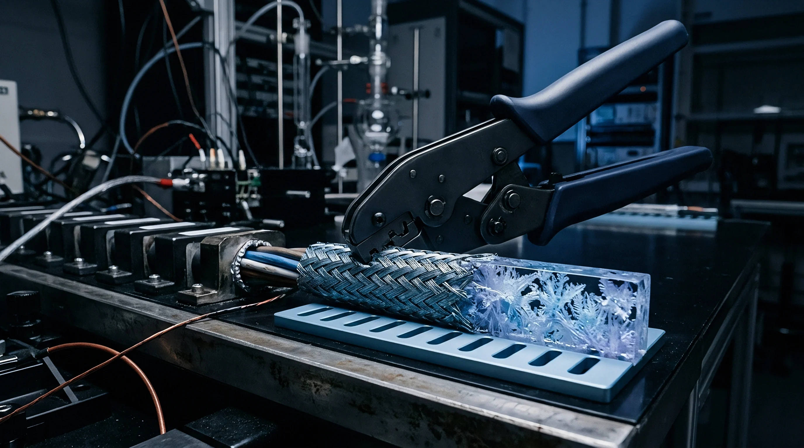
Validating Maxwell series parameters under cryogenic thermal ramps introduces severe measurement challenges. Liquid nitrogen injection chambers generate strong convection currents, thermal micro-oscillations, and frost accumulation on optical windows, while sub-ambient mechanical testing demands strict isolation of load cell signal chains from freezing temperature gradients.
Testing rigid polymers down to 77 K requires sub-micron displacement resolution under thermal swings spanning over 200 K. Load frames must compensate for structural frame contraction during long test sequences; without dynamic frame compensation, thermal contraction of test grips appears incorrectly as mechanical strain within test specimen data.
| Uncertainty Parameter | Magnitude at 293 K | Magnitude at 77 K | Traceability Standard / Method |
|---|---|---|---|
| Load Cell Thermal Drift | ±0.05% Full Scale | ±0.45% Full Scale | Direct Thermal Isolation Bridge Calibration |
| Frame Thermal Contraction | < 0.2 microns | 14.8 microns | In-situ Laser Interferometry Measurement |
| Temperature Sensor Gradient | ±0.1 K | ±1.2 K | Calibrated Platinum Resistance Thermometer (IEC 60751) |
| Displacement Gauge Resolution | ±5.0 nanometers | ±12.0 nanometers | Capacitive Gage Dual-Probe System |
Contact extensometers used at 77 K can slip or induce local stress concentrations on glass-hard polymer surfaces. Non-contact techniques like Digital Image Correlation avoid contact issues but suffer when frost builds up on optical windows. Nitrogen purging of outer optical enclosures prevents moisture condensation, maintaining line-of-sight imaging fidelity across 300 K to 77 K ramps.
Thermal lag between internal specimen cores and surface-mounted temperature sensors introduces systematic error during fast ramps. Thermal lag exceeds 8 K in 4 mm thick epoxy specimens cooled at 10 K per minute. Fitting Prony series parameters against surface thermistor logs shifts the apparent relaxation spectrum along the temperature axis, distorting calculated activation energies.
Systematic thermal lag between specimen core and surface thermistors causes artificial broadening of calculated relaxation spectra during fast thermal ramps.
Mechanical compliance of cryostat load frames varies non-linearly over wide temperature ranges. Load cell calibrations performed at 23 °C lose accuracy when conductive paths cool internal sensor flexures. Differential capacitive gages mounted directly onto specimen gauge lengths eliminate external machine compliance from raw load-displacement datasets.
Test fixture clamp pressure fluctuates during cooling because of thermal contraction mismatches between metallic grips and polymeric samples. Insufficient grip force permits micro-slippage during stress relaxation sweeps. Excessive clamping force induces localized transverse compressive strain, altering measured axial relaxation dynamics through multi-axial stress coupling.

DMA and TMA Protocols for Viscoelastic Parameter Extraction
Multi-frequency Dynamic Mechanical Analysis provides the master curves needed to fit high-order Maxwell parameters. DMA applies sinusoidal strain at fixed frequencies while stepping or ramping temperature across material transition zones. Time-Temperature Superposition principles allow shifting frequency sweeps horizontally along the logarithmic time axis to construct master curves spanning twelve to fifteen decades of time.
Thermomechanical Analysis tracks linear thermal expansion coefficients across sub-ambient ramps. Slope discontinuities in TMA length-versus-temperature plots mark glass transition limits and secondary sub-ambient transition thresholds. Precise expansion coefficient inputs are vital for separating pure thermal strain from viscoelastic relaxation responses during dynamic modeling.
Parameter fitting involves non-linear least squares optimization algorithms to extract Maxwell modulus weights and relaxation times from experimental dynamic storage and loss modulus curves:
E'(omega) = E_infinity + Sum_{i=1}^{N} (E_i omega^2 tau_i^2) / (1 + omega^2 tau_i^2)
E”(omega) = Sum_{i=1}^{N} (E_i omega tau_i) / (1 + omega^2 tau_i^2)
Optimization routines tend to encounter ill-conditioned system matrices when fitting more than five Maxwell branches simultaneously. Tikhonov regularization suppresses numerical oscillations in extracted spectrum parameters, enforcing smooth weight distributions across relaxation time decades.
Cryogenic DMA testing requires multi-frequency sweeps executed at tight temperature increments, typically 2 K steps, with minimum ten-minute thermal equilibration holds per step. Continuous temperature ramping during DMA creates thermal gradients that shift loss factor peak positions; steady-state stepped temperature sweeps remain essential for qualifying critical flight hardware.

Calibration
Traceability Chains and Sensor Uncertainty Budgets
Ensuring structural reliability of cryogenic components requires metrological traceability across all measurement equipment utilized during material calibration sequences. Temperature sensors, force transducers, and displacement measurement instruments must trace back through unbroken chains of certified calibration standards to national metrology institutes. Measurement uncertainty propagation dictates the final confidence bound on predicted stress values inside high-value finite element structural simulations.
Platinum resistance thermometers serve as the primary reference accuracy across sub-ambient thermal runs. Calibrated per IEC 60751 standard procedures, calibrated sensors achieve baseline temperature uncertainties within ±0.03 K at 273.15 K and ±0.08 K at 77.3 K. Using standard uncalibrated thermocouples introduces errors up to ±3.5 K at cryogenic temperatures, corrupting shift factor parameters and invalidating lifetime predictions.
Force measurement during long-term stress relaxation tests requires low-drift signal conditioning. Sub-ambient load cells require signal conditioning hardware optimized for micro-volt drift stability over multi-day test windows. Bridge excitation voltages must remain stable within ±0.002% to prevent thermal self-heating errors inside sub-ambient test chambers.
| Uncertainty Component | Standard Uncertainty u_i | Probability Distribution | Sensitivity Coefficient c_i | Uncertainty Contribution (MPa) |
|---|---|---|---|---|
| Specimen Cross-Section Area | 0.012 mm² | Normal | -3.2 MPa/mm² | 0.0384 |
| Load Cell Force Calibration | 0.15 N | Normal | 0.80 MPa/N | 0.1200 |
| Displacement Sensor Drift | 0.04 microns | Rectangular | 4.5 MPa/micron | 0.1039 |
| Temperature Control Error | 0.25 K | Normal | 1.85 MPa/K | 0.4625 |
| Thermal Shift Factor Fit | 0.03 (log units) | Normal | 8.4 MPa/unit | 0.2520 |
Summing these contributions in quadrature yields a combined standard uncertainty of approximately ±0.55 MPa on an initial glassy modulus measurement of 4200 MPa. Applying a coverage factor of k = 2 expands the reported uncertainty interval to ±1.10 MPa at a 95% confidence level. Temperature control errors represent the dominant component of overall model parameter uncertainty.
Evaluating long-term calibration stability takes continuous tracking of reference standard drift histories over multi-year service cycles. Laboratory reference sensors undergo re-calibration every twelve months to catch subtle calibration shifts caused by thermal shock aging of internal sensor elements. Unmonitored sensor drift degrades baseline measurements, introducing hidden systemic risk into safety-critical aerospace stress verifications.

How to Verify Model Predictions against Physical Test Bench Results?
Validating a fitted Generalized Maxwell model requires comparing numerical finite element predictions against dynamic thermal ramp test datasets not included during parameter calibration steps. Verification protocols test material samples under complex multi-step thermal ramps containing simultaneous displacement holds and force relaxation tracking sequences.
The verification sequence runs a multi-stage thermal profile while recording reaction forces on a constrained test coupon:
The experiment begins by cooling the specimen from 293 K to 150 K at a constant cooling rate of 5 K per minute under fixed end-displacement conditions. Force sensors record thermal strain accumulation combined with simultaneous stress relaxation. The system holds temperature at 150 K for 120 minutes to observe isothermal relaxation behavior, followed by reheating back to 293 K at 2 K per minute to measure residual stress recovery paths.
Model validation criteria demand that predicted stress values remain within calculated experimental uncertainty bands across the entire test duration. Discrepancies exceeding total measurement uncertainty indicate missing physical phenomena within the constitutive framework, such as unmodeled structural relaxation, stress-dependent non-linear viscoelasticity, or micro-cracking damage accumulation.
Comparing predicted stress trajectories against bench data reveals the operating boundaries of thermorheological simplicity assumptions. Where experimental stress curves deviate from model predictions during rapid thermal ramps, non-linear stress-assisted shift mechanisms must replace standard linear shift equations inside the numerical solver.
Acceptance testing of structural adhesive batches relies on standardized verification protocols to certify compliance with engineering stress limits. A batch fails qualification if measured stress relaxation rates fall below designated lower tolerance bounds during cryogenic thermal hold periods. Strict calibration tracking prevents false rejections caused by measurement tool drift during verification runs.
Documenting verification outcomes requires clear separation between measurement uncertainties, material batch variance, and model formulation errors. Calibration dossiers retain raw sensor calibration files, raw voltage outputs, environmental log files, and processed strain fields to back up compliance claims during third-party design audits.
Dossier

Verification Protocols and Quality Management Integration
Integrating cryogenic viscoelastic material models into production engineering pipelines requires formalized quality control procedures and qualification documentation. Engineering teams relying on Maxwell model parameters for structural integrity checks must mandate traceably calibrated test dossiers for every material batch entering assembly operations. Raw material suppliers must deliver standardized material dossiers confirming baseline thermomechanical property consistency across production runs.
Standardized qualification procedures define acceptable tolerance bands for Prony series parameters across incoming material lots. Modulus weights E_i must hold within ±5% of nominal design baselines, while shift factor activation energies must demonstrate consistency within ±3%. Material lots exceeding these limits introduce uncontrolled thermal stress variations in finalized structural components.
- Material Lot Certification ~ Document raw chemical batch numbers, resin stoichiometric ratios, cure cycle temperature logs, and post-cure glass transition thermal signatures.
- Calibration Instrument File ~ Maintain ISO/IEC 17025 accredited calibration certificates for all dynamic mechanical analyzers, load cells, thermistors, and optical gages used during parameter extraction.
- Raw Test Data Archive ~ Store unedited multi-frequency DMA storage and loss curves, TMA thermal expansion traces, and step-temperature hold datasets in raw binary formats.
- Prony Optimization Audit Log ~ Record objective function convergence histories, Tikhonov regularization parameters, shift factor fitting residual errors, and verified parameter sets.
- Bench Model Validation Report ~ Include dynamic thermal ramp verification test comparisons, spatial thermal gradient measurements, and uncertainty band overlay plots.
Quality management systems built around ISO 9001 and AS9100 standards mandate regular audit trails covering computational material models. Model parameters stored inside finite element material databases require write-protection controls and strict version tracking to prevent unauthorized parameter substitution during design iterations. Changing a single Maxwell relaxation time constant without documented re-verification revokes component design approvals.
Recalibration protocols for testing hardware protect against hidden measurement drift in long-term qualification programs. Load frames subjected to repeated cryogenic thermal cycles undergo alignment checks every six months to verify coaxial loading geometry. Angular misalignment exceeding 0.05 degrees introduces localized bending moments, distorting measured axial relaxation dynamics.
Procurement specifications for cryogenic adhesives and structural components mandate verified relaxation limits. Skipping vendor verification risks field failures driven by unexpected low-temperature embrittlement or thermal stress cracking. Complete material dossiers provide the metrological backing required to defend structural safety margins under rigorous spaceflight qualification standards.
Contractual agreements between material vendors and system integrators specify exact testing standards, reference environmental conditions, and maximum allowed model parameter tolerances. Non-compliant material batches face immediate rejection prior to structural integration, protecting program schedules and engineering budgets from downstream quality failures.