Quantifying Hydrostatic Pressure and Thermal Cross Sensitivity Shifts in Marine Sensor Calibration Matrices
Cross-sensitivity matrix calibration corrects temperature-dependent pressure errors in marine sensors, securing depth measurement accuracy across full ocean depth.
Deformation
Mechanical strain and structural deflection govern how marine pressure transducers behave in the deep ocean. When a piezoresistive silicon, resonant quartz, or capacitive ceramic sensor descends from surface conditions to abyssal depths reaching 70 MPa, hydrostatic pressure compresses the transducer body. At the same time, ambient water temperatures fall from up to 35 °C at equatorial surfaces to -2 °C in polar or benthic zones.
These effects act together: hydrostatic compression shifts the crystalline lattice geometry and material stiffness of the sensing diaphragm, altering both its thermal expansion coefficient and the temperature coefficient of Young’s modulus.
In a Grade 5 titanium housing, Young’s modulus is roughly 114 GPa at 20 °C, dropping by about 0.04 percent for every degree Celsius increase. As hydrostatic pressure squeezes the housing, unequal expansion between the metal casing, internal fill fluid, and sensing element generates cross-axis stress fields. Left uncompensated, this cross-sensitivity causes depth errors over 5 meters at a profiling depth of 6000 meters.
For a 70 MPa titanium-housed silicon strain sensor, a 0.015 percent full-scale accuracy rating depends on a 12-point calibration performed in a 20 °C oil bath; that rating degrades to 0.08 percent full-scale if a thermal gradient over 0.5 °C per minute forms across the housing during vertical profiling.

Coupled Mechanical and Thermal Strain Response
Hydrostatic loads exert uniform normal stress on transducer membranes, compressing microscopic sensing elements and changing their electrical resistivity or resonant frequencies. Temperature shifts alter baseline dimensions and electrical carrier mobility in piezoresistive strain gauges. Because these physical responses couple, temperature sensitivity changes with applied pressure, and pressure sensitivity varies with temperature.
Standard linear temperature compensation models break down in deep water because the cross-coupling term scaled by both pressure and temperature becomes large relative to overall measurement tolerances.
Piezoresistive silicon strain gauges bonded to isolated diaphragms show strong cross-sensitivity because piezoresistive coefficients depend heavily on temperature. As pressure compresses the silicon crystal, these coefficients drop, changing the output voltage span generated per unit of applied pressure. At the same time, thermal expansion mismatches between the silicon substrate, glass bonding layers, and metal housing introduce localized shear stresses that shift the zero-pressure baseline and distort the pressure response non-linearly across the ocean’s thermal envelope.
Titanium Grade 5 sensor housings experience a thermal expansion shift of 0.0012 percent span per degree Celsius at hydrostatic pressures exceeding 40 MPa.

Zero Point Offset Drift under Pressure
Baseline shifts at zero applied pressure usually stem from thermal relaxation in internal fill fluids and mechanical seals. High hydrostatic loads force molecules in oil-filled sensors into tighter packing, raising fluid viscosity and bulk modulus. When temperature fluctuates, the volumetric expansion of this compressed silicone oil creates a hydraulic bias against the sensing diaphragm, shifting the baseline zero point.
Thermal gradients shift internal component alignment, while the spatial distribution of primary strain mechanisms across marine pressure sensor assemblies reveals distinct environmental vulnerabilities.
- Diaphragm Radial Compression induces localized stress concentrations that alter piezoresistive element resistance independently of applied fluid force.
- Housing Volumetric Contraction squeezes internal fluid reservoirs, generating parasitic internal hydraulic pressure variations across ambient thermal ranges.
- Piezoresistive Substrate Thermal Mismatch generates interfacial shear forces between silicon chips and glass pedestals, shifting sensor zero-point offsets.
- Fill Fluid Compressibility Variation alters internal hydraulic stiffness, changing the mechanical transfer function between external seawater pressure and internal sensing elements.
| Housing Alloy | Young’s Modulus (GPa) | Expansion Coefficient (10^-6 / K) | Thermal Modulus Shift (% / °C) | Pressure Sensitivity Shift (% FS / MPa) |
|---|---|---|---|---|
| Titanium Grade 5 | 114 | 8.6 | -0.040 | 0.0012 |
| Inconel 718 | 205 | 13.0 | -0.028 | 0.0008 |
| Monel K-500 | 179 | 13.7 | -0.035 | 0.0015 |
| Hastelloy C-276 | 205 | 11.2 | -0.031 | 0.0010 |
| Fused Silica | 73 | 0.5 | +0.012 | 0.0001 |
Ignoring structural strain cross-coupling during deep-sea profiling corrupts oceanographic density calculations, leading directly to buoyancy control failures in autonomous underwater vehicles.


Mapping
Multivariable surface equations provide the mathematical framework needed to decouple hydrostatic pressure readings from thermal interference in ocean sensors. Older calibration methods relied on separate one-dimensional adjustments: a pressure polynomial set sensitivity at room temperature, and a temperature polynomial corrected for thermal zero drift. In deep water, these isolated models leave systematic residual errors because cross-coupling terms are neglected.
Accurately modeling sensor behavior requires a continuous two-dimensional surface function that treats pressure and temperature as joint independent variables.
A standard two-dimensional calibration model defines corrected hydrostatic pressure as a bivariate polynomial of raw signal output and temperature readings. The surface fit incorporates raw bridge output voltage, temperature diode signal, and a matrix of cross-sensitivity coefficients. Building this matrix requires selecting polynomial degrees high enough to capture non-linear physical behavior without triggering numerical oscillations near the edges of the operational envelope.

Polynomial Surface Fitting Formulations
Bivariate sensor calibrations typically use polynomial orders from third to fifth degree in pressure, combined with second to fourth degree in temperature. While higher polynomial orders improve curve-fitting precision across laboratory test points, going too high triggers Runge’s phenomenon, creating artificial pressure oscillations between calibration data points.
Evaluating bivariate calibration equations relies on structured matrix algebra. Raw sensor outputs form an observation matrix, while reference pressures and temperatures establish the target vector. A linear least-squares fit then calculates the coefficient matrix by minimizing residual pressure errors across all environmental test points.
Higher-order cross-terms reflect specific physical interactions, including the thermal coefficient of pressure sensitivity and the pressure coefficient of thermal expansion.
Inverting poorly conditioned cross-sensitivity matrices amplifies digital voltage noise into false depth fluctuations at deep ocean equilibrium.
Matrix Inversion and Numerical Stability
Solving cross-sensitivity matrices requires careful numerical conditioning. Standard Vandermonde matrices built from raw voltage and temperature powers carry high condition numbers, often exceeding 10^10. Inverting an ill-conditioned matrix introduces severe round-off errors under standard floating-point arithmetic.
Keeping condition numbers manageable requires normalizing raw sensor signals and temperature inputs to dimensionless values between -1 and +1 before constructing matrix terms. Using Singular Value Decomposition or QR factorization isolates near-singular components and stabilizes inversion, lowering condition numbers below 10^3 to preserve numerical precision throughout the processing steps.
High-order surface polynomials require calibration test points distributed evenly across the operational envelope to prevent numerical instability at combined temperature and pressure extremes.

Chamber
Temperature-controlled hyperbaric test vessels supply the environmental conditions needed to build accurate calibration matrices. Characterizing cross-sensitivity requires applying precise hydrostatic pressures up to 70 MPa while maintaining fluid bath temperatures between -2 °C and 35 °C. The test setup pairs an automated liquid-immersion temperature bath with a high-precision hydraulic deadweight tester or pressure controller, preserving traceable reference standards over multi-day calibration runs.
Establishing stable reference conditions inside pressure chambers presents severe thermodynamic challenges. Rapidly compressing hydraulic fluids generates adiabatic heating within the vessel, raising internal temperatures by up to 1.5 °C per 10 MPa increment in mineral oil systems or 0.2 °C per 10 MPa in water-based systems. As a result, the chamber must dwell at each target pressure point until internal thermal equilibrium settles back within 0.005 °C of the set bath temperature.

Hyperbaric Temperature Controlled Test Apparatus
Liquid bath immersion systems surrounding the hyperbaric vessel require active circulation to eliminate spatial temperature gradients across the chamber. A temperature variation of just 0.05 °C across a sensor housing creates internal thermal stresses that shift piezoresistive bridge balance and generate flawed calibration coefficients. Primary pressure measurements rely on working deadweight testers calibrated against national metrological standards, with expanded measurement uncertainties below 0.005 percent of reading.
Passing electrical signal lines through hyperbaric vessel walls introduces stray thermal electromotive forces (EMF) at wire feedthrough junctions. Temperature differences between internal chamber fluid and ambient laboratory air produce Seebeck voltages across metal feedthrough pins. Standard multi-conductor copper feedthroughs generate up to 0.4 microvolts per degree Celsius of temperature differential, adding measurable offset errors to high-resolution bridge signals.
Using low-thermal feedthrough connectors and differential signal conditioning amplifiers minimizes this thermal noise.
Adherence to ISO/IEC 17025 calibration criteria mandates logging active temperature stability within 0.005 °C prior to acquiring pressure reference signals.

Thermal Equilibrium and Transient Settling Times
Rapid fluid compression during testing requires strict settling protocols before recording sensor data. The thermal time constant of a thick-walled titanium pressure vessel in a liquid bath ranges from 15 to 45 minutes, depending on vessel geometry and fluid agitation speed. Attempting to shorten calibration cycles by recording data during thermal relaxation skews matrix coefficients by misattributing transient thermal stress to static pressure sensitivity.
Execution of a rigorous hyperbaric thermal calibration requires a systematic sequence of environmental steps across the entire operational envelope.
- Mount the target pressure sensor inside the hyperbaric vessel and connect low-thermal signal feedthrough lines to high-precision digital multimeters.
- Submerge the hyperbaric vessel into the fluid bath and set temperature control to the lowest target calibration point, typically -2.00 °C.
- Maintain thermal bath control until internal chamber temperature sensors confirm equilibrium stability within 0.005 °C over a 20-minute dwell window.
- Apply hydraulic pressure in discrete increments from atmospheric zero to maximum rating, pausing at each step for thermal dissipation.
- Log stable reference pressure, raw sensor bridge output voltage, and internal sensor temperature diode readings at every pressure plateau.
- Depressurize the chamber back to atmospheric zero to record hysteresis baseline signals under cold thermal conditions.
- Step bath temperature upward to the next calibration plateau, repeating the pressure step sequence across all target temperature points.
Relying on ambient thermal stabilization during rapid pressure stepping without active fluid heating and cooling control fails to provide sufficient accuracy for deep-sea sensor calibration.


Coefficients
Evaluating cross-coupling parameters requires building complete measurement uncertainty budgets according to standard metrological protocols. Every coefficient in a bivariate calibration matrix carries an individual uncertainty derived from reference sensor tolerances, environmental stability limits, fitting residuals, and signal noise floors. Propagating these parameter uncertainties through matrix inversion determines the total expanded uncertainty of depth calculations under operational sea conditions.
Mechanical degradation under cyclic loading alters the elastic response of sensor diaphragms, altering calibration coefficients over time. Silicon-to-glass bond lines, internal lead-wire solder joints, and elastomeric seals experience viscoelastic relaxation during repeated deep pressure cycles, producing gradual drift in thermal offset parameters.
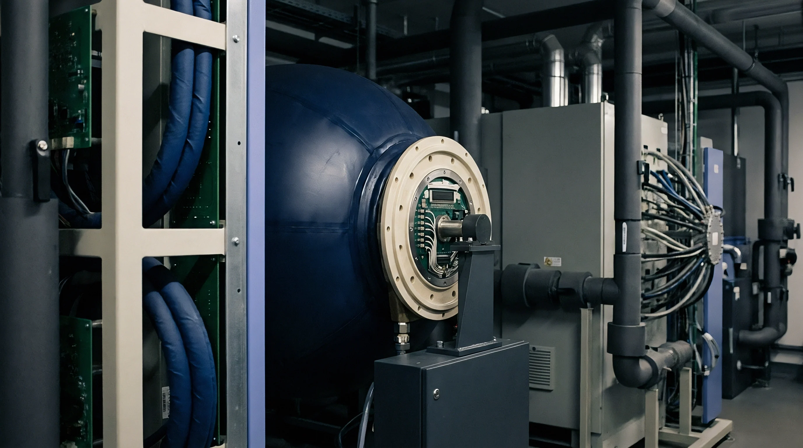
Uncertainty Budget Propagation in Matrix Inversion
Standard measurement variances propagate from raw readings to calculated pressure through partial derivative sensitivity coefficients. For a matrix polynomial model, finding depth uncertainty requires taking the partial derivative of pressure with respect to each matrix term, raw signal voltage, and temperature reading. Combined standard uncertainty equals the square root of the sum of squared derivative-weighted input variances, plus covariance terms between correlated fitting parameters.
Consider a worked calculation for a marine pressure sensor operating at 6000 meters depth (60.000 MPa applied pressure) and 2.00 °C seawater temperature. The sensor uses a second-order bivariate matrix calibration model defined by P = C10 S + C01 (T – T0) + C11 S (T – T0) + C20 S^2, where S is raw signal voltage (volts), T is temperature (°C), T0 is reference temperature (20.0 °C), and Cij represent matrix coefficients.
Assume the measured parameters and primary coefficients for this calculation:
- Raw Bridge Signal S equals 4.80000 V at 60.000 MPa, with measurement uncertainty u(S) equal to 0.00005 V.
- Temperature Reading T equals 2.00 °C with reference T0 equal to 20.00 °C, yielding delta T equal to -18.00 °C, with measurement uncertainty u(T) equal to 0.01 °C.
- Primary Sensitivity C10 equals 12.5000 MPa/V with fitting uncertainty u(C10) equal to 0.0005 MPa/V.
- Thermal Offset C01 equals -0.01200 MPa/°C with fitting uncertainty u(C01) equal to 0.00008 MPa/°C.
- Cross Term C11 equals -0.00250 MPa/(V·°C) with fitting uncertainty u(C11) equal to 0.00003 MPa/(V·°C).
- Non-Linearity Term C20 equals 0.00100 MPa/V^2 with fitting uncertainty u(C20) equal to 0.00001 MPa/V^2.
Evaluating pressure yields P = (12.5000 × 4.80000) + (-0.01200 × -18.00) + (-0.00250 × 4.80000 × -18.00) + (0.00100 × 4.80000^2) = 60.0000 + 0.2160 + 0.2160 + 0.0230 = 60.4550 MPa. Evaluating partial derivatives with respect to inputs gives the sensitivity factors: dP/dS = C10 + C11(T – T0) + 2 C20 S = 12.5000 + 0.0450 + 0.0096 = 12.5546 MPa/V; dP/dT = C01 + C11 S = -0.0120 – 0.0120 = -0.0240 MPa/°C.
Summing variance contributions gives u(P)^2 = (12.5546 × 0.00005)^2 + (-0.0240 × 0.01)^2 + (4.80000 × 0.0005)^2 + (18.00 × 0.00008)^2 + (-86.40 × 0.00003)^2 + (23.04 × 0.00001)^2 = 0.00000039 + 0.00000006 + 0.00000576 + 0.00000207 + 0.00000672 + 0.00000005 = 0.00001505 MPa^2. Taking the square root yields combined standard uncertainty u(P) = 0.00388 MPa. Multiplying by a coverage factor k = 2 produces an expanded uncertainty of 0.00776 MPa, equivalent to roughly 0.78 meters of depth error at 6000 meters.
An annual drift figure of 0.005 percent full-scale per year for fused-quartz pressure sensors rests on continuous pressure loading tests conducted over 1000 hours at 15 °C. This figure changes if cyclic deep excursions between 0 and 60 MPa exceed 500 cycles annually as mechanical hysteresis accumulates in housing mounting welds. Furthermore, the long-term thermal cross-sensitivity shift coefficient of 1.8 × 10^-6 full-scale per degree Celsius per year across multi-year subsea deployments cannot be fully defended because long-term hyperbaric aging data over 36 consecutive months remains sparse in published literature. Under this specific uncertainty, a buyer specifies dual redundant sensor packages or schedules annual calibration casts to bound zero drift.
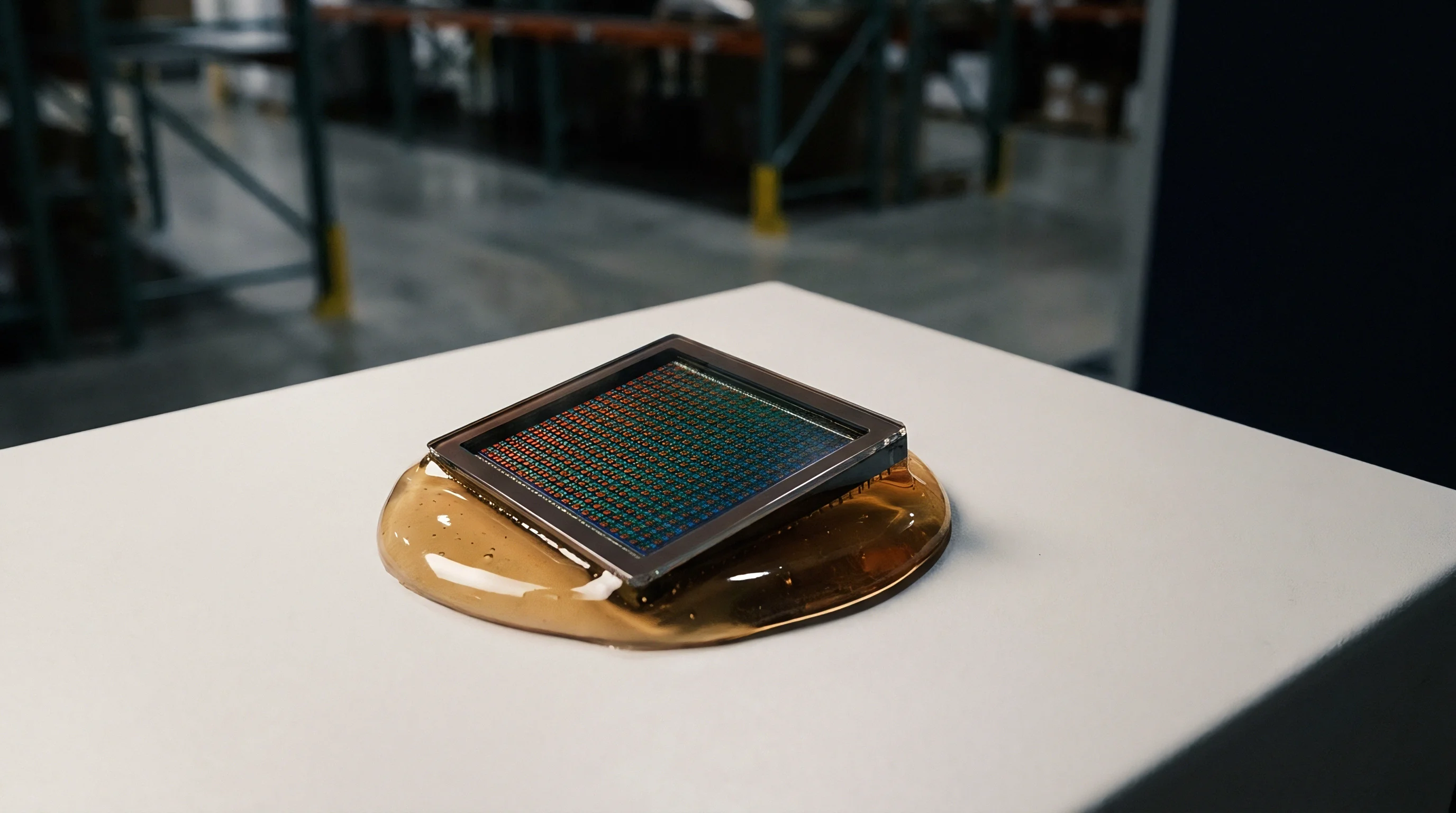
Does Cyclic Pressure Fatigue Alter Temperature Compensation Coefficients?
Repeated pressure loading down to abyssal depths introduces microscopic dislocations within crystalline silicon diaphragms and metallic isolation housings. Cyclic mechanical stress combined with prolonged exposure to cold temperatures alters the internal baseline strain distribution, gradually degrading calibrated thermal compensation terms. Operational drift analysis shows that thermal offset parameters shift faster than primary pressure sensitivity terms during long-term ocean deployments.
Verification protocols must systematically validate vendor calibration dossiers before deploying instruments into high-consequence subsea applications.
- Traceability Scope Verification confirms that calibration references carry accredited ISO/IEC 17025 certification covering the full temperature and pressure ranges.
- Residual Error Surface Audit inspects matrix fitting residual plots for systematic non-random error distributions that indicate polynomial underfitting.
- Hysteresis Bound Analysis evaluates offset signal differences between increasing and decreasing pressure paths across all test temperatures.
- Condition Number Evaluation checks normalized matrix inversion conditioning metrics to prevent digital signal noise amplification during processing.
| Uncertainty Source | Standard Variance Value | Probability Distribution | Sensitivity Coefficient | Uncertainty Contribution (MPa) |
|---|---|---|---|---|
| Primary Pressure Reference | 0.0015 MPa | Normal (k=1) | 1.000 | 0.00150 |
| Temperature Reference Measurement | 0.0050 °C | Normal (k=1) | 0.024 MPa/°C | 0.00012 |
| Matrix Surface Fitting Residual | 0.0022 MPa | Rectangular | 1.000 | 0.00127 |
| Raw Signal ADC Quantification Noise | 0.00003 V | Rectangular | 12.55 MPa/V | 0.00022 |
| Thermal Bath Spatial Non-Uniformity | 0.0080 °C | Rectangular | 0.024 MPa/°C | 0.00011 |
| Viscoelastic Sensor Creep Shift | 0.0030 MPa | Rectangular | 1.000 | 0.00173 |
Thermal excursion hysteresis causes lingering zero-point offsets long after the transducer returns to sea-surface conditions.
How microscopic viscoelastic relaxation within glass-passivated silicon strain diaphragm bonds alters matrix cross-terms over multi-year deep sea deployments remains an unresolved question in long-term sensor metrology.


Recalibration
Managing financial planning for subsea sensor fleets requires balancing the high cost of hyperbaric matrix calibration against the risk of measurement drift during offshore operations. A full bivariate matrix calibration across 16 to 25 pressure-temperature equilibrium points takes 48 to 72 hours of continuous chamber time, generating service costs between $3,500 and $6,000 per sensor. By contrast, a simplified single-point temperature offset check costs roughly $300, but fails to detect shifts in higher-order cross-sensitivity coefficients.
Evaluating financial trade-offs requires determining whether operational sensor drift exceeds maximum permissible depth measurement errors during deployment intervals.

Interval Optimization and Drift Thresholds
Setting sensor maintenance on fixed time intervals often causes premature servicing of stable instruments or prolonged operation of drifting units. Risk-based calibration scheduling uses historical drift data to project when individual matrix coefficients will breach acceptable tolerances. Sensors deployed on deep ocean moorings for 12 to 24 months show non-linear drift during the first 90 days, followed by linear long-term zero drift.
In-situ field validation provides a practical way to check sensor matrix stability without pulling instruments from subsea infrastructure. Oceanographic research vessels run deep CTD (Conductivity, Temperature, Depth) casts using rosette samplers equipped with reference sensors and water sampling bottles. Comparing deep-water pressure readings against reference instruments at abyssal depths yields a verification point that separates zero-offset drift from cross-sensitivity shifts.
| Calibration Method | Chamber Test Points | Dwell Time (Hours) | Unit Service Cost (USD) | Residual Error at 6000m (Meters) | Cross-Term Drift Risk Coverage |
|---|---|---|---|---|---|
| 1-Point Atmospheric Zero Trim | 1 | 1 | $300 | 4.50 | Uncovered |
| 1D Pressure Recalibration (20 °C) | 6 | 8 | $1,200 | 1.80 | Partial |
| Full 2D Bivariate Matrix Recalibration | 20 | 60 | $4,500 | 0.25 | Full |
| In-Situ Deep CTD Co-Location Cast | 1 | 12 | $800 | 1.20 | Uncovered |
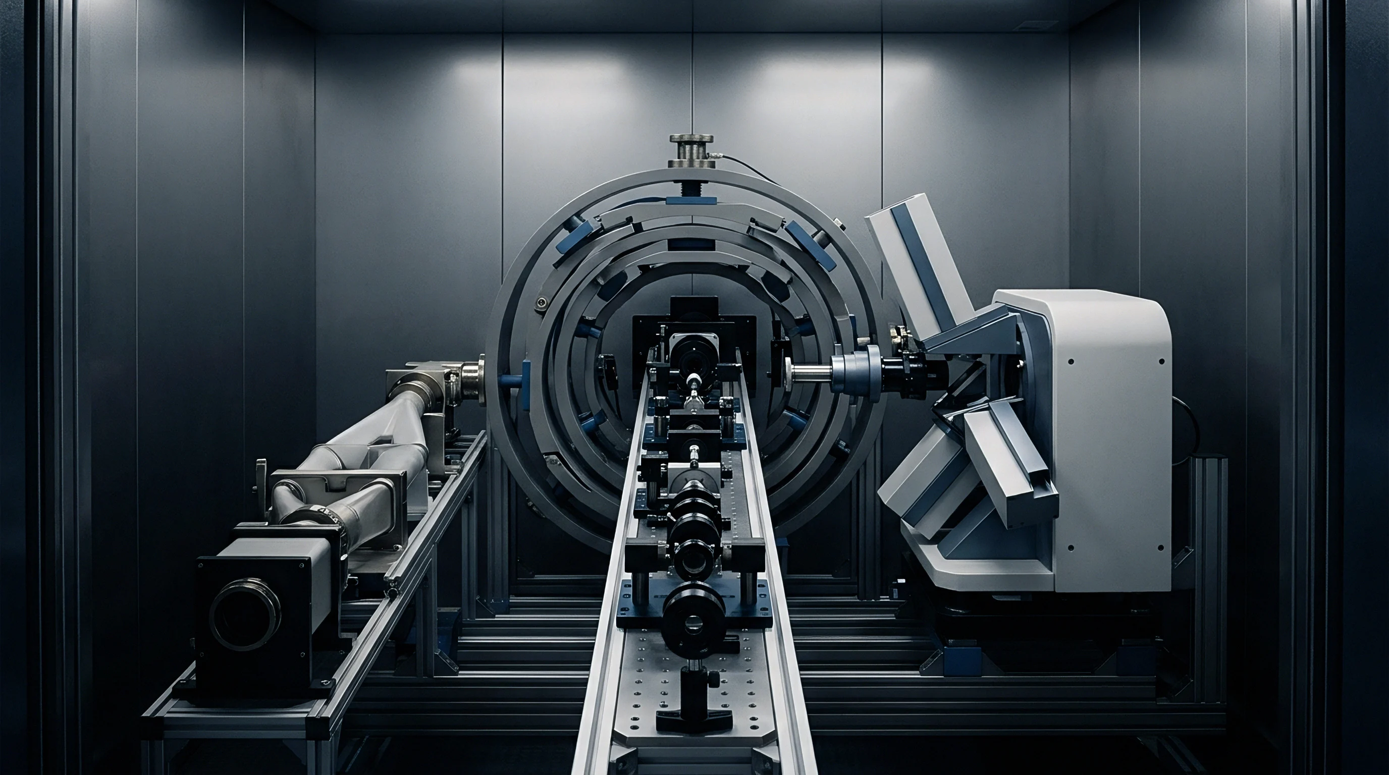
Commercial Dossier and Accreditation Verification
Reviewing calibration documentation from third-party laboratories requires strict verification of technical competence. Accredited facilities must provide documentation detailing calibration measurement capability (CMC) uncertainties for combined pressure and temperature test points. A certificate reporting isolated pressure uncertainty without stating temperature chamber stability invalidates the traceability chain for deep ocean operations.
Contracts for subsea sensor servicing incorporate standard quality assurance clauses governing calibration interval adjustments based on statistical control limits. ISO 10012 clause 7.1.2 mandates that measurement management systems systematically evaluate historical drift data to shorten calibration intervals when sensor drift exceeds 80 percent of specified operational tolerance thresholds.