Analytical Error Bounds in Static Leveling and Gyrocompassing Systems
Analytical error bounds combine accelerometer bias tilt projection and latitude secant gyrocompassing equations to establish deterministic spatial uncertainty limits.

Vector

Gravitational and Rotational Vector Field Sensitivity
Precision alignment demands rigid reference frames. Static leveling and gyrocompassing rely on two invariant environmental vector fields available to a ground-based platform: local gravitational acceleration and Earth’s rotational velocity. Local gravity provides a downward vector perpendicular to the geoid with an average magnitude of 9.81 meters per second squared.
Earth rotates around its spin axis at an angular velocity of 7.292115 x 10⁻⁵ radians per second, equivalent to 15.04107 degrees per hour. Static leveling determines pitch and roll by resolving the direction of the gravity vector relative to the body axes of an inertial measurement unit. Static gyrocompassing determines geographic heading by sensing the horizontal component of the Earth rotation rate vector.
The analytical error bounds of these system operations stem directly from the mathematical projection of sensor measurement uncertainties onto these reference vector fields.
Platform orientation uses a localized North-East-Down coordinate frame. In this geographic frame, the local gravity vector aligns strictly with the Down axis, represented as T. The Earth rotation vector sits in the North-Down plane, defined by latitude, containing a horizontal component equal to Earth rate multiplied by the cosine of latitude and a vertical component equal to Earth rate multiplied by the sine of latitude.
When an inertial measurement unit sits at a tilt angle relative to the horizontal plane, the orthogonal accelerometers record fractional components of gravity. Concurrently, orthogonal gyroscopes resolve fractions of the Earth rotation vector. Gravity provides an absolute physical vector.
Measuring these projections allows the host computer to solve for roll, pitch, and yaw through deterministic trigonometric relations.
Sensor errors disturb these geometric calculations. Accelerometer bias, scale factor errors, and sensor axis misalignment distort the measured gravity vector, introducing direct errors into the calculated pitch and roll angles. Similarly, gyroscope bias drift, angle random walk, and cross-axis coupling corrupt the measured rotational rate vector.
The mathematical link between sensor level errors and attitude error bounds relies on partial derivative sensitivity equations. For small angular offsets, small changes in accelerometer readings yield proportional tilt errors inversely related to local gravitational acceleration. Small changes in gyroscope outputs yield azimuth errors inversely related to both Earth rotation rate and local latitude cosine.
Coordinate Frame Transformations and Vector Perturbations
Transformation from the sensor body frame to the geographic local-level frame uses a directional cosine matrix derived from roll, pitch, and heading angles. Sensor body accelerations match the matrix product of the directional cosine matrix and the reference gravity vector when the platform remains completely stationary. Static leveling assumes zero external linear acceleration.
Any non-gravitational acceleration, such as localized structural vibration or foundation swaying, directly corrupts the static gravity measurement. A uncompensated residual acceleration of 1 millig along a horizontal sensor axis introduces an artificial tilt error of approximately 1 milliradian, or 3.44 arcminutes.
Vector perturbation analysis quantifies system degradation under combined sensor imperfections. Let the measured acceleration vector equal the true body gravity projection corrupted by a static bias vector, a scale factor matrix, and non-orthogonal axis alignment factors. Resolving pitch and roll requires isolating the horizontal accelerometer outputs.
Small angle approximations show that pitch error equals the x-axis acceleration error divided by gravity, while roll error equals the y-axis acceleration error divided by gravity. The baseline sensitivity factor for static leveling is 102 micro-g per arcsecond. Achieving arcsecond-level leveling accuracy demands accelerometer bias stability and noise levels significantly below this threshold.
Orthogonality errors destroy coordinate transformations. If the orthogonal axes of a triaxial accelerometer cluster deviate from absolute 90-degree alignment by 0.1 milliradians, acceleration along the z-axis couples directly into the horizontal x and y channels. Because the z-axis accelerometer experiences the full 1-g gravitational vector in near-level conditions, a 0.1 milliradian alignment error transfers 100 micro-g of fictitious acceleration into the horizontal calculations.
This geometric cross-coupling generates an uncompensated tilt error of 20.6 arcseconds. Calibration procedures must isolate non-orthogonality matrices from sensor bias through multi-position tumble testing before calculating operational leveling bounds.
Analytical bounds on gyrocompassing depend on the horizontal projection of Earth rate. The north-pointing gyroscope measures Earth rate multiplied by the cosine of latitude, while the east-pointing gyroscope theoretically measures zero rotation rate when aligned with geographic north. Misalignment in pitch or roll tilts the east-pointing gyroscope into the vertical plane, causing it to pick up a component of the larger vertical Earth rotation rate.
This tilt-induced rate coupling creates heading calculation errors that grow larger as geographic latitude increases toward the poles.


Tilt
Accelerometer Error Model Derivations
Analytical bounds for static leveling rest on the detailed mathematical error model of the accelerometers. The output signal of an accelerometer channel includes deterministic bias, thermal bias drift, scale factor instability, second-order non-linearity, axis cross-coupling, and sensor noise. Accelerometer bias mimics physical platform tilt.
The primary static pitch error equation expands to account for these specific error contributions:
delta_theta = (b_x + s_xx f_x + k_xx f_x^2 + delta_alpha_xy f_y + delta_alpha_xz f_z + n_x) / g
In this relationship, delta_theta represents pitch calculation error in radians, b_x represents x-axis accelerometer zero-g bias in meters per second squared, s_xx represents scale factor error, k_xx represents quadratic acceleration non-linearity, delta_alpha_xz represents mechanical misalignment of the x-axis toward the z-axis, and n_x represents broad-band sensor noise. Under near-level static conditions, f_x and f_y remain near zero, while f_z approaches 1 g. The general pitch error equation simplifies to delta_theta = (b_x + delta_alpha_xz g + n_x) / g.
This simplified form highlights that horizontal zero-g bias and vertical axis misalignment represent the dominant mathematical error mechanisms in static leveling operations.
A zero-g offset stability of 50 micro-g over a 24-hour window limits static leveling uncertainty to 10.3 arcseconds at room temperature.
Scale factor non-linearity distorts tilt calculations. While scale factor errors have minimal impact on horizontal accelerometers experiencing zero acceleration near level, they significantly affect off-level leveling applications. When a platform sits at a steep slope of 15 degrees, the horizontal accelerometer experiences a gravity projection of 0.2588 g.
Under these conditions, a scale factor error of 500 parts per million introduces an acceleration error of 129.4 micro-g. This acceleration offset generates an additional tilt calculation error of 26.7 arcseconds. High-precision leveling systems requiring wide operating tilt ranges must implement full high-order polynomial scale factor compensation in host software.

Tilt Error Bounds under Cross Axis Coupling
Cross-axis coupling arises from fabrication tolerances in MEMS structures and mechanical mounting inaccuracies in quartz-flexure accelerometers. Sensor cross-axis coupling introduces synthetic acceleration. When the mounting plane of a triaxial accelerometer cluster deviates from the platform body frame, multi-axis error propagation occurs.
Resolving roll angle under combined errors follows a similar formulation to pitch, where y-axis acceleration errors divide by local gravity. If the x-axis and y-axis share mutual non-orthogonality, the tilt calculations become coupled, requiring simultaneous matrix inversion to extract true platform orientation.
The total analytical error bound for static leveling uses a Root-Sum-Square combination for uncorrelated noise sources and direct summation for worst-case systematic calibration residuals. Evaluating the error budget across temperature demands mapping thermal coefficient terms. A high-grade capacitive MEMS accelerometer exhibits a thermal bias coefficient of roughly 20 micro-g per degree Celsius.
Operating across a temperature variation of 15 degrees Celsius without real-time thermal compensation creates a bias drift of 300 micro-g. This thermal shift degrades static leveling accuracy by 61.8 arcseconds, exceeding the error allowances of tactical-grade alignment systems.
Quantization noise in the sensor conditioning electronics sets the ultimate resolution limit of static leveling. A 16-bit analog-to-digital converter operating over a full-scale acceleration range of +/- 2 g provides a quantization step size of 61 micro-g per least significant bit. This quantization coarse graining limits individual tilt resolution to 12.6 arcseconds.
Upgrading the signal chain to a 24-bit delta-sigma converter reduces the quantization step size to 0.238 micro-g per bit, shifting the baseline performance floor from converter quantization to the physical noise density of the accelerometer sensor element.
The following error mechanisms systematically degrade horizontal tilt determination accuracy:
- Zero-g Bias Instability shifts accelerometer output offsets over time, creating false horizontal acceleration readings that directly map to tilt errors.
- Cross-Axis Alignment Deviation couples vertical gravitational forces into horizontal measurement channels, generating tilt calculation errors proportional to platform elevation.
- Thermal Coefficient Coefficients drive temperature-dependent bias shifts across operational gradients, requiring real-time sensor housing compensation.
- Second-Order Acceleration Non-Linearity distorts output signals under static g loads, introducing skew into steep-angle leveling solutions.
Evaluating these error parameters against target leveling bounds requires structured parameter bounds. The baseline operational boundaries in Table 1 quantify how typical component performance figures convert into static tilt errors.
| Accelerometer Parameter | Tactical Grade Specification | Navigation Grade Specification | Derived Pitch/Roll Error (Tactical) | Derived Pitch/Roll Error (Navigation) |
|---|---|---|---|---|
| Zero-g Offset Bias | 1.0 mg | 25 micro-g | 206.2 arcseconds | 5.1 arcseconds |
| Bias Thermal Drift (-40C to +85C) | 0.5 mg | 10 micro-g | 103.1 arcseconds | 2.0 arcseconds |
| Axis Non-Orthogonality | 0.5 mrad | 0.05 mrad | 103.1 arcseconds | 10.3 arcseconds |
| Scale Factor Uncertainty | 500 ppm | 50 ppm | 26.7 arcsec (at 15 deg tilt) | 2.7 arcsec (at 15 deg tilt) |
| In-Run Bias Instability | 50 micro-g | 5 micro-g | 10.3 arcseconds | 1.0 arcseconds |
Platform mounting compliance interacts directly with accelerometer performance. Bending or warping of the circuit board mounting structure under gravitational loading alters the physical alignment of the sensor axes relative to the platform baseplate. A mechanical deflection of just 5 micrometers across a 50-millimeter sensor package substrate changes the physical tilt angle by 20.6 arcseconds.
Uncompensated structural flexibility sets an insurmountable lower bound on static leveling performance regardless of accelerometer calibration quality.
Precision static leveling calculations rely on precise horizontal accelerometer offsets rather than absolute vertical gravity magnitudes.


Heading
Mathematical Formulations for Earth Rate Gyrocompassing
Static gyrocompassing extracts geographic heading by measuring the vector components of Earth’s rotation rate using high-precision gyroscopes. Earth rotation defines the heading reference. Assuming a perfectly leveled platform, the horizontal gyroscopes measure north and east components of the Earth rate vector.
The north-axis gyroscope registers Omega_N = Omega cos(phi) cos(psi), while the east-axis gyroscope registers Omega_E = -Omega cos(phi) sin(psi), where Omega is Earth rotation rate, phi is local latitude, and psi is geographic heading angle relative to true north. Computing heading uses the arctangent of the ratio between east and north measured rotation rates:
psi = -arctan(omega_E / omega_N)
Analytical error propagation for true north determination is derived by taking the total differential of this heading equation with respect to gyroscope bias errors and platform tilt errors. The expanded analytical heading error equation reveals the critical dependencies governing gyrocompassing uncertainty:
delta_psi = (b_gy cos(psi) + b_gx sin(psi)) / (Omega cos(phi)) + delta_theta tan(phi) + delta_phi tan(phi) tan(psi)
In this expression, delta_psi represents total azimuth error in radians, b_gx and b_gy represent in-run bias errors of the x-axis and y-axis gyroscopes, Omega is Earth rate, phi is local latitude, delta_theta is pitch calculation error, and delta_phi is roll calculation error. This formulation demonstrates two severe physical amplification factors: the latitude secant multiplier 1 / cos(phi) operating on gyroscope bias, and the latitude tangent multiplier tan(phi) operating on leveling residual errors.
Under ISO 26262 functional safety audits, uncompensated gyro scale factor asymmetry introduces non-recoverable azimuth drift during stationary alignment.
Small gyroscope bias errors generate substantial heading errors. At a latitude of 45 degrees, the horizontal Earth rate component Omega cos(45 deg) equals 10.635 degrees per hour, or 0.1856 milliradians per hour. A gyroscope with an uncompensated horizontal bias error of 0.01 degrees per hour introduces an azimuth error of delta_psi = 0.01 / 10.635 = 0.00094 radians, or 3.23 arcminutes.
Achieving a 1-arcminute static heading error bound at mid-latitudes demands horizontal gyroscope bias stability better than 0.0031 degrees per hour.
Why Does High Latitude Degrade Gyrocompassing Azimuth Accuracy?
Polar latitudes degrade azimuth resolution severely. As latitude phi approaches 90 degrees, the cosine of latitude approaches zero, causing the term 1 / (Omega cos(phi)) to approach infinity. At 0 degrees latitude (the equator), the horizontal Earth rate reaches its maximum of 15.041 degrees per hour.
At 60 degrees latitude, horizontal Earth rate drops to 7.520 degrees per hour, doubling the azimuth sensitivity to gyroscope bias errors. At 80 degrees latitude, horizontal Earth rate decreases to 2.612 degrees per hour, multiplying azimuth sensitivity by a factor of 5.76 relative to the equator.
Tilt coupling exacerbates high-latitude gyrocompassing degradation. The pitch tilt error term delta_theta tan(phi) maps leveling errors directly into heading errors. At 60 degrees latitude, tan(60 deg) equals 1.732.
A static leveling pitch error of 1 arcminute (17.5 microradians) multiplies by 1.732, adding 1.732 arcminutes of false heading error. At 85 degrees latitude, tan(85 deg) equals 11.43, causing a 1-arcminute pitch leveling error to generate 11.43 arcminutes of azimuth error. High-latitude gyrocompassing demands exceptional leveling accuracy to prevent vertical Earth rate components from swamping horizontal rate measurements.
Gyroscope performance tiers dictate the ultimate feasibility of static gyrocompassing. Tactical-grade MEMS gyroscopes with bias stabilities around 1.0 degree per hour cannot accomplish static gyrocompassing, as the sensor bias dwarfs the 15.04 degree per hour total Earth rate vector. Tactical optical gyroscopes achieve bias stabilities between 0.1 and 0.01 degrees per hour, enabling coarse gyrocompassing accuracy within 0.5 to 2 degrees.
Navigation-grade Fiber Optic Gyroscopes (FOG) and Ring Laser Gyroscopes (RLG) with bias stabilities between 0.001 and 0.005 degrees per hour deliver arcminute to sub-arcminute static heading accuracy.
Executing static gyrocompassing follows a strict mathematical procedure with specific error propagation risks at each stage:
- Leveling Baseline Initialization computes platform pitch and roll using static accelerometer gravity vector sensing, where residual tilt directly scales the subsequent vertical Earth rate coupling.
- Earth Rate Sample Accumulation integrates horizontal gyroscope outputs over a defined stationary window, where gyroscope angle random walk sets the decreasing noise variance floor.
- Quad-Position Indexing Drift Suppression rotates the sensor package through 90-degree or 180-degree physical increments, canceling static gyroscope bias errors from the azimuth calculation.
- Azimuth Calculation Synthesis computes geographic heading through arctangent projection, applying local latitude scale adjustments to lock the final directional solution.
Performance ceilings vary sharply across sensor modalities. Table 2 details the latitude-dependent analytical error bounds generated by different gyroscope technologies.
| Gyroscope Technology | In-Run Bias Stability | Angle Random Walk (ARW) | Heading Error at 0 deg Latitude | Heading Error at 60 deg Latitude | Heading Error at 80 deg Latitude |
|---|---|---|---|---|---|
| High-End MEMS | 0.05 deg/hr | 0.015 deg/sqrt(hr) | 11.47 arcminutes | 22.95 arcminutes | 66.08 arcminutes |
| Tactical FOG | 0.01 deg/hr | 0.003 deg/sqrt(hr) | 2.29 arcminutes | 4.59 arcminutes | 13.22 arcminutes |
| Navigation FOG | 0.001 deg/hr | 0.0005 deg/sqrt(hr) | 0.23 arcminutes (13.8 sec) | 0.46 arcminutes (27.5 sec) | 1.32 arcminutes (79.3 sec) |
| Strategic RLG | 0.0002 deg/hr | 0.0001 deg/sqrt(hr) | 0.046 arcminutes (2.8 sec) | 0.092 arcminutes (5.5 sec) | 0.26 arcminutes (15.8 sec) |
Selecting an inadequate gyroscope bias specification for high-latitude alignment operations results in total directional divergence, rendering autonomous platform heading identification impossible.

Clamp
Mechanical Creep and Fixture Distortion Mechanics
Analytical bounds derived from ideal mathematical models fail when physical mounting structures yield under thermal or mechanical stress. Mechanical creep produces false angular rates. Mounting hardware, sensor packages, and baseplate interface clamps undergo continuous micro-strain when subjected to temperature changes, mechanical fasteners torque loads, and structural bending forces.
Physical distortion of the sensor enclosure shifts the structural alignment of the sensor axes relative to the platform reference frame, creating non-gravitational and non-rotational measurement signals.
Mechanical creep in aluminum mounting structures proceeds through strain relaxation. When an aluminum sensor bracket clamps onto a platform frame using steel bolts, differential thermal expansion generates continuous shear stresses across the interface. Over extended stationary periods, these stress gradients cause microscopic slip events and material deformation.
A physical angular drift rate of just 0.001 degrees per hour caused by structural housing creep registers directly on a navigation-grade gyroscope. The system host cannot distinguish this mechanical creep rate from true Earth rotation, contaminating the static gyrocompassing solution.
Thermal gradients across an aluminum sensor mounting bracket cause structural bending that mimics accelerometer tilt drift.
Baseplate strain coupling distorts internal sensor elements. External loads applied to a platform chassis transmit mechanical strain through mounting bosses into the sensor enclosure substrate. Quartz flexure accelerometers and MEMS sensing structures experience stress-induced changes in internal element gaps.
An internal mechanical strain of 10 micro-strain across a MEMS accelerometer die alters the capacitive pickoff gap balance, producing an artificial zero-g bias shift of up to 100 micro-g. This structural bias shift degrades leveling calculations independently of electronic performance limits.
Thermal Gradient Induced Structural Warping
Thermal gradients generate structural bending moments. Uniform temperature changes expand or contract mounting fixtures symmetrically, which can be compensated using static polynomial calibration tables. Non-uniform thermal gradients across the sensor package break structural symmetry, inducing mechanical bowing and angular warping.
A temperature difference of 0.1 degree Celsius across opposite sides of a 100-millimeter aluminum mounting block creates a differential thermal expansion of 0.23 micrometers. This localized expansion tilts the sensor mounting surface by 0.47 arcseconds.
Dynamic thermal transients accentuate gradient-induced structural warping. When ambient temperature changes rapidly, heat propagates through the outer enclosure toward the inner sensor housing at rates governed by material thermal conductivity and heat capacity. Transient thermal gradients induce localized material strain, causing the sensor frame to flex continuously during the thermal transient state.
Accelerated thermal testing shows that dynamic thermal slopes of 1.0 degree Celsius per minute generate temporary structural tilt shifts exceeding 15 arcseconds. These transient errors persist until the entire sensor assembly reaches thermal equilibrium.
Verifying the mechanical decoupling and structural stability of a static sensor installation requires a rigorous physical inspection routine:
- Mount the sensor assembly onto a vibration-isolated optical bench inside a climate-controlled enclosure using calibrated torque wrenches on all fasteners.
- Establish baseline static leveling and rate outputs over a 4-hour thermal equilibrium period at a constant reference temperature.
- Apply a controlled thermal step change of 10 degrees Celsius to the ambient chamber air while logging sensor baseplate mechanical strain gauges and housing temperature profiles.
- Measure angular deviation between the sensor housing reference mirror and the bench reference cube using a dual-axis optical autocollimator.
- Quantify residual mechanical hysteresis by returning the chamber to the initial reference temperature and recording permanently settled structural offset shifts.
Supplier technical documentation frequently attributes unaccounted baseline drift to environmental vibration rather than acknowledging structural creep inside their low-cost housing assemblies.

Window

Allan Variance Decomposition for Stationary Filtering
Time-domain signal processing sets the achievable lower bound of sensor noise in static leveling and gyrocompassing systems. Integration time reduces high frequency noise. Stationary signal acquisition allows filtering algorithms to average out zero-mean stochastic noise processes.
Sensor noise is not purely white; stochastic noise characteristics shift across integration time windows. Allan variance analysis decomposes sensor noise into specific stochastic components, identifying the exact integration window required to achieve optimal measurement bounds.
Allan variance plots identify five distinct noise mechanisms that affect static measurement systems: angle random walk (or velocity random walk for accelerometers), bias instability, rate random walk, rate ramp, and quantization noise. Allan variance identifies deterministic noise boundaries. At short integration times, high-frequency white noise dominates the signal variance, causing the Allan deviation curve to decrease with a slope of -0.5 on a log-log plot.
Averaging signals over longer time windows effectively attenuates white noise, improving sensor measurement resolution.
Bias instability defines the absolute performance floor for stationary signal averaging. As integration time increases, the Allan deviation curve reaches a minimum plateau where flicker noise dominates the system response. Beyond this optimal integration time, long-term drift mechanisms such as rate random walk (slope +0.5) and thermal rate ramps (slope +1.0) begin to corrupt the signal.
Averaging data past the Allan variance minimum point increases overall measurement error rather than reducing it. Identifying the minimum point of the Allan variance curve establishes the maximum permissible static averaging window.
Optimal Integration Windowing and Sampling Limits
Determining the optimal integration window for static gyrocompassing requires balancing angle random walk suppression against in-run bias instability growth. Angle random walk generates heading uncertainty that scales inversely with the square root of integration time T. The statistical heading uncertainty contribution from ARW follows the equation:
sigma_psi_ARW = ARW / (sqrt(T) Omega cos(phi))
Where ARW represents gyroscope angle random walk in degrees per sqrt(hour), T represents integration time in hours, Omega represents Earth rotation rate, and phi represents latitude. Integrating a navigation-grade FOG with an ARW of 0.001 deg/sqrt(hr) over a 60-second window (0.0166 hours) at 45 degrees latitude yields an ARW-induced heading uncertainty of sigma_psi_ARW = 0.001 / (sqrt(0.0166) 10.635) = 0.000728 radians, or 2.50 arcminutes. Extending the integration window to 600 seconds (0.166 hours) reduces this white noise contribution to 0.79 arcminutes.
Higher sampling rates increase signal bandwidth. High-speed sampling above the Nyquist rate prevents high-frequency environmental vibrations from aliasing into the low-frequency passband of the static filter. Anti-aliasing filters must provide high attenuation at frequencies corresponding to mechanical resonance modes of the platform structure.
Digital low-pass filtering applied to high-rate sampled data converts high-frequency vibration energy into predictable statistical variance, which yields to time-domain averaging filters.
Quantization noise limits static leveling accuracy when the analog to digital converter resolution drops below 20 effective bits.
Optimizing static integration windows requires systematic filtering configuration rules:
- Stationary Window Duration must match the Allan variance minimum time floor to prevent long-term flicker noise from degrading baseline calculations.
- Anti-Aliasing Filter Cutoff must sit below half the digital sampling frequency to prevent mechanical vibration modes from folding into static band measurements.
- Stationary Motion Detection must continuously monitor high-frequency acceleration variance to discard data frames contaminated by base movement.
- Quantization Noise Margin must exceed the target sensor noise density by a factor of four to preserve signal chain resolution integrity.
Whether real-time adaptive windowing algorithms can reliably distinguish between low-frequency geophysical microseismics and internal sensor bias drift without external reference aiding remains an open engineering question.

Budget
Analytical Error Budget Integration Mechanics
Constructing a complete analytical error budget for static leveling and gyrocompassing systems requires integrating every physical, electrical, and mathematical uncertainty source into a unified statistical framework. Budget allocations require strict statistical modeling. Systematic errors with known physical bounds sum linearly under worst-case analysis.
Uncorrelated stochastic errors combine through Root-Sum-Square (SRSS) formulations. The total system error budget equations define spatial uncertainty bounds for pitch, roll, and true heading angles.
Total pitch uncertainty combines accelerometer bias, axis alignment deviations, electrical noise, thermal drift, and mechanical fixture flexing. The unified pitch error expression is written as:
sigma_theta_total = sqrt( (sigma_b_acc / g)^2 + (sigma_align_acc)^2 + (sigma_noise_acc / (g sqrt(T)))^2 + (sigma_flexure)^2 ) + |delta_theta_cal_residual|
In this expression, sigma_b_acc represents uncompensated accelerometer zero-g bias stability, sigma_align_acc represents mechanical sensor axis non-orthogonality uncertainty, sigma_noise_acc represents accelerometer velocity random walk, T represents integration filtering time, sigma_flexure represents mechanical baseplate structural bending, and delta_theta_cal_residual represents deterministic calibration residual error. Achieving a sub-10-arcsecond total leveling error bound requires constraining each constituent variance term to strict sub-micro-g or sub-arcsecond limits.
Total heading uncertainty combines the unified pitch error, horizontal gyroscope bias instability, angle random walk, scale factor asymmetry, and latitude geometry multipliers. The complete gyrocompassing heading error budget expression takes the expanded form:
sigma_psi_total = sqrt( (sigma_b_gyro / (Omega cos(phi)))^2 + (ARW / (sqrt(T) Omega cos(phi)))^2 + (sigma_theta_total tan(phi))^2 + (sigma_sf_gyro tan(psi))^2 ) + |delta_psi_cal_residual|
This integrated equation highlights how tilt errors sigma_theta_total feed directly into the azimuth uncertainty calculation through the latitude tangent coupling multiplier. Leveling uncertainty dominates heading accuracy at high latitudes.
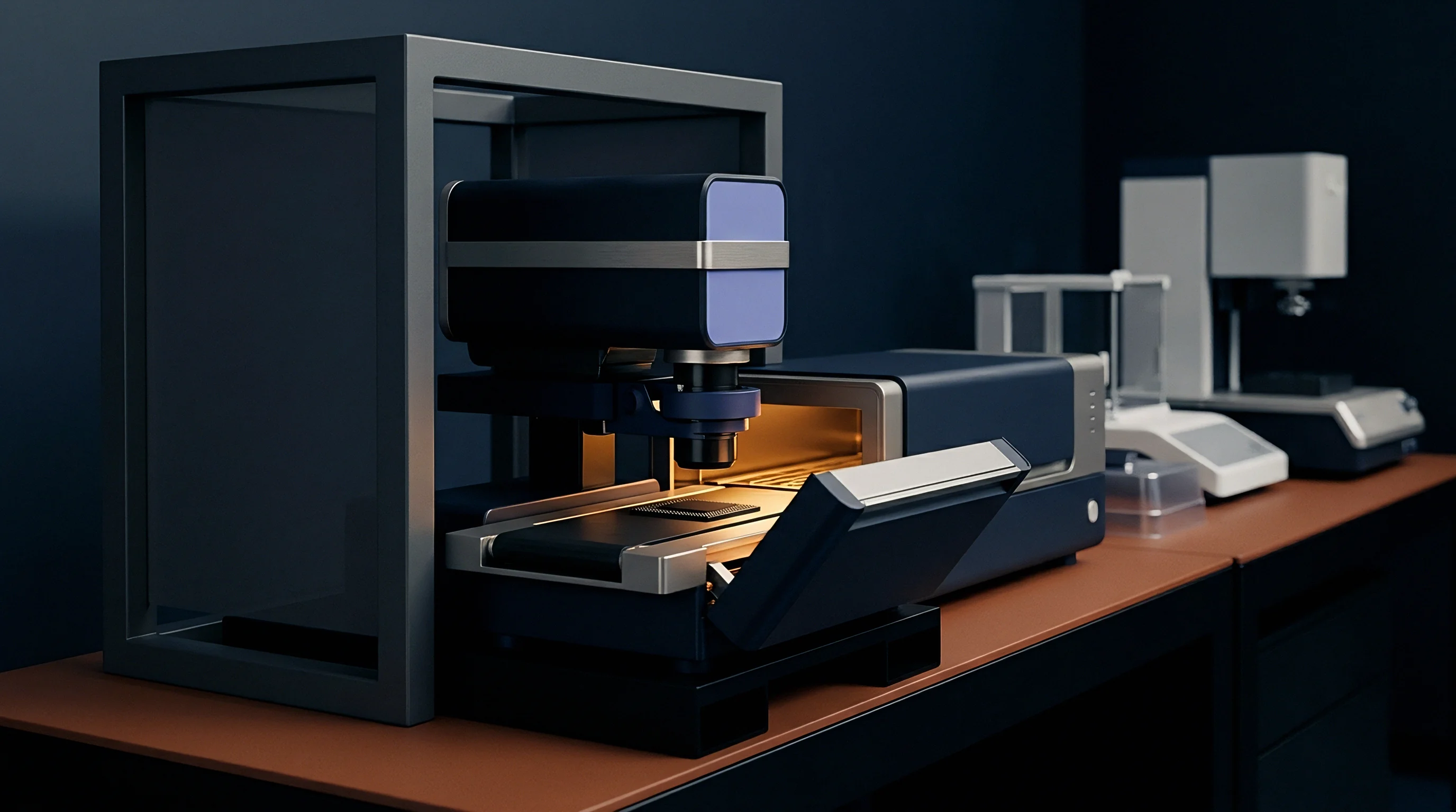
Performance Ceilings across Sensor Modalities
Comparing physical sensor modalities exposes trade-offs between unit cost, physical volume, power dissipation, and achievable error bounds. Calibration reduces repeatable thermal offset errors. MEMS inertial sensors offer small form factors, low power consumption, and low unit costs, but their relatively high bias drift and thermal sensitivity restrict their performance to tactical leveling and coarse gyrocompassing applications.
Optical gyroscopes (FOG and RLG) deliver high bias stability and low angle random walk, providing the physical baseline for high-precision navigation-grade gyrocompassing systems.
Fiber optic gyroscopes eliminate mechanical friction. FOG technology uses Sagnac interference inside a closed fiber coil to measure angular rotation, providing exceptional scale factor linearity and low noise density. Ring Laser Gyroscopes offer superior bias stability but require dither mechanisms to overcome lock-in phenomena at ultra-low rotation rates.
Quartz flexure accelerometers provide high stability and low thermal drift for gravity vector sensing, remaining the baseline standard for high-precision static leveling applications.
System architects evaluate error budget allocation frameworks against target performance classes. Table 3 outlines the comprehensive error budgets required to hit tactical, navigation, and strategic alignment tiers.
| Error Source Sub-Component | Tactical System (Target: 1 deg Azimuth) | Navigation System (Target: 0.1 deg Azimuth) | Strategic System (Target: 0.01 deg Azimuth) |
|---|---|---|---|
| Accelerometer Zero-g Bias | 1.0 mg (206 arcsec tilt) | 0.05 mg (10.3 arcsec tilt) | 0.005 mg (1.0 arcsec tilt) |
| Accelerometer Thermal Drift | 0.5 mg (103 arcsec tilt) | 0.02 mg (4.1 arcsec tilt) | 0.002 mg (0.4 arcsec tilt) |
| Gyroscope In-Run Bias | 0.1 deg/hr | 0.005 deg/hr | 0.0003 deg/hr |
| Gyroscope Angle Random Walk | 0.02 deg/sqrt(hr) | 0.001 deg/sqrt(hr) | 0.0001 deg/sqrt(hr) |
| Mechanical Mounting Bending | 30 arcseconds | 5 arcseconds | 0.5 arcseconds |
| Integration Window Required | 60 seconds | 300 seconds | 1200 seconds |
| Latitude Ceiling for Spec | 45 degrees | 70 degrees | 85 degrees |
Standard procurement contract line items based on MIL-STD-810H Method 514.8 mandate that static leveling and gyrocompassing analytical error bounds must be validated under continuous ambient micro-vibration profiles, shifting qualification compliance from pure static laboratory conditions to real-world industrial environments.