Multi Axis Tumble Matrix Error Model Non Linear Optimization Calibration
Multi-axis tumble matrix optimization extracts 21 sensor parameters, reducing vector error residuals to native sensor noise bounds.

Tumble
Calibrating multi-axis inertial sensor triads relies on the local gravity vector as an exact physical magnitude standard. Exposing a triaxial accelerometer array to a structured sequence of static spatial orientations produces a system of equations where total vector magnitude equals one local gravity unit. Rate tables or multi-axis indexing heads rotate the sensor package through predetermined tilt angles, simultaneously exciting primary sensitivity axes and cross-coupling channels.
Static multi-position calibration schedules vary in orientation count, which directly sets how well spatial error components can be observed. A basic six-position tumble profile aligns each orthogonal axis parallel and antiparallel to local vertical, offering enough independent constraints to solve three primary zero-g bias offsets and three linear scale factors. Expanding the matrix to 12, 24, or 36 orientations adds oblique tilt angles that reveal inter-axis non-orthogonality, package assembly misalignments, and higher-order scale factor terms.
| Profile Density | Orientation Count | Primary Orientation Angles (deg) | Observable Parameters | Spatial Vector Uniformity |
|---|---|---|---|---|
| Basic Hexahedral | 6 | 0, 90, 180, 270 on orthogonal planes | Bias (3), Linear Scale Factors (3) | Coarse (Axis-aligned only) |
| Dodecahedral Grid | 12 | Orthogonal plus 45-degree oblique planes | Bias (3), Scale Factors (3), Misalignments (6) | Moderate (Planar diagonals) |
| Icosahedral Matrix | 20 | Vertices of regular icosahedron frame | Bias (3), Scale Factors (6), Misalignments (6) | High (Spherically distributed) |
| Extended Octahedral | 24 | 15-degree pitch and roll steps with full yaw | Bias (3), Scale (3), Misalignment (6), Quadratic (3), Cross-Terms (6) | Very High (Dense spherical mesh) |
Running an extended tumble matrix requires static stability at each indexing position. Vibration from motor drives or lab bench movement violates the static equilibrium assumption, corrupting the calibration dataset with dynamic acceleration noise. Processing pipelines typically sample raw digital output over a fixed dwell time, using finite impulse response filtering or averaging windows to extract steady-state readings.
A 24-position tumble profile isolates cross-axis accelerometer misalignment to within 0.02 millirad when ambient fixture thermal drift remains below 0.1 kelvin per hour.
Sequencing errors during physical tumble manipulation degrade parameter estimation. The following sequence establishes a 12-position static orientation routine for triaxial sensor arrays:
- Mounting fixture leveling aligns the base rotation plane with local horizontal within 0.005 degrees using electronic precision bubble levels.
- Axis zeroing reference aligns the primary internal sensor frame with the mechanical datum of the multi-axis indexing head.
- Orthogonal face exposures record steady-state output vectors across all six cardinal orientations for 30 seconds per station.
- Oblique angle indexing rotates the inner gimbal frame through 45-degree pitch and roll steps to generate multi-axis vector combinations.
- Reversed trajectory execution repeats the spatial rotation sequence in reverse order to identify thermal hysteresis and mechanical backlash in the positioning rig.
Truncating a tumble matrix to speed up production throughput creates unresolvable coupling between cross-axis misalignment and non-linear scale factors. Sourcing sensor modules calibrated under undersampled tumble schedules exposes downstream guidance algorithms to uncompensated orientation errors that compound linearly over navigation time.

Mapping
Mathematical models of sensor imperfection transform raw ADC outputs into calibrated physical measurements. The classical linear transformation uses a three-by-three matrix of scale factors and cross-axis alignments added to a three-element bias vector. MEMS fabrication tolerances, packaging stresses, and sensing element non-linearities require extended models that include higher-order polynomial terms and g-sensitivity parameters.
A full 21-parameter non-linear physical model accounts for quadratic scale factor curvature, cross-axis coupling, and structural bias shifts. The accelerometer vector equation models observed acceleration against true input acceleration using explicit expansion terms:
Output = Bias + (Scale Factor Matrix) (Misalignment Matrix) Input + (Quadratic Matrix) Input^2 + Noise
Gyroscope error modeling introduces extra complexity due to acceleration-sensitive bias shifts, known as g-sensitivity. Silicon capacitive MEMS gyroscopes contain proof masses that deflect under linear acceleration, altering the resonant gap and mimicking angular velocity signals. The comprehensive error model integrates a three-by-three g-sensitivity matrix directly into the rate vector transformation, requiring simultaneous tilt and rotation profiles during tumble sequences.
IEEE 1293 compliance demands explicit declaration of third-order scale factor non-linearities whenever sensor operating ranges exceed ten times the linear calibration threshold.
Cross-axis sensitivity stems from physical assembly misalignments and electrical coupling between adjacent readout channels. Silicon photolithography places sensing structures on a single die with high precision, but die-attach adhesive curing and IC packaging strain introduce package tilt relative to substrate pins. A complete mapping framework models package non-orthogonality separately from internal die non-orthogonality, decoupling mechanical mounting errors from internal sensor physics.
Factory single-axis tumble sweeps are often assumed to provide sufficient calibration for multi-axis applications. That assumption ignores internal cross-axis stress coupling induced when thermal gradients and mounting torque act along secondary axes simultaneously. Omitting higher-order non-linear cross-terms from the model specification leaves uncompensated residuals that ruin dead-reckoning accuracy during high-g maneuvering.
Solver
Determining optimal parameter values for a 21-parameter error model requires non-linear least-squares optimization. The objective function minimizes squared differences between observed sensor vector magnitude and the known gravitational magnitude across all tumble positions. Iterative optimization engines adjust bias, scale factor, and non-orthogonality parameters until residual scalar error converges to a global minimum.
Which Solver Algorithm Prevents Local Minima Traps?
The Levenberg-Marquardt algorithm combines gradient descent with the Gauss-Newton approach, providing robust convergence for multi-axis sensor calibration models. When initial parameter estimates lie far from the global minimum, the solver behaves like gradient descent, stepping safely down the error surface. As residual error shrinks, it transitions smoothly toward Gauss-Newton speed, achieving quadratic convergence near the optimal solution.
To demonstrate solver mechanics, consider a calibration dataset collected from a triaxial MEMS accelerometer array subjected to a 24-position tumble profile. Initial parameter estimates start with zero bias, unity scale factors, and zero cross-axis misalignments. The local gravitational magnitude standard is 9.80665 m/s^2.
Initial uncalibrated vector magnitude error across the dataset yields a sum of squared residuals of 4.25 x 10^-2 (m/s^2)^2.
During iterations 1 through 4, the solver dynamically adjusts the damping factor lambda to navigate steep parameter gradients, updating primary bias offsets and main-diagonal scale factors. Sum of squared residuals drops to 1.12 x 10^-4 (m/s^2)^2. Iterations 5 through 8 refine off-diagonal misalignment terms and second-order quadratic terms, fine-tuning the parameter Jacobian matrix.
Sum of squared residuals falls to 3.85 x 10^-7 (m/s^2)^2. Iterations 9 through 12 achieve convergence criteria, where step-size parameter changes fall below 1.0 x 10^-12, reaching a final residual sum of squares of 1.78 x 10^-7 (m/s^2)^2 as sensor noise limits further refinement.
Damping parameters in trust-region algorithms protect non-linear optimizations from premature divergence when initial sensor bias estimates carry significant error.
Solving non-linear calibration models introduces divergence risks when parameter spaces exhibit mathematical ill-conditioning. Sparse tumble matrices that omit oblique tilt frames cause near-singularities in the Jacobian matrix, leading to unconstrained scaling parameters. Enforcing parameter bounds through constrained trust-region reflective algorithms prevents numerical instability during optimization.
Whether non-linear solvers can consistently separate structural packaging strain from internal die non-linearities without absolute position feedback from external optical encoders remains open to debate.
Fixture
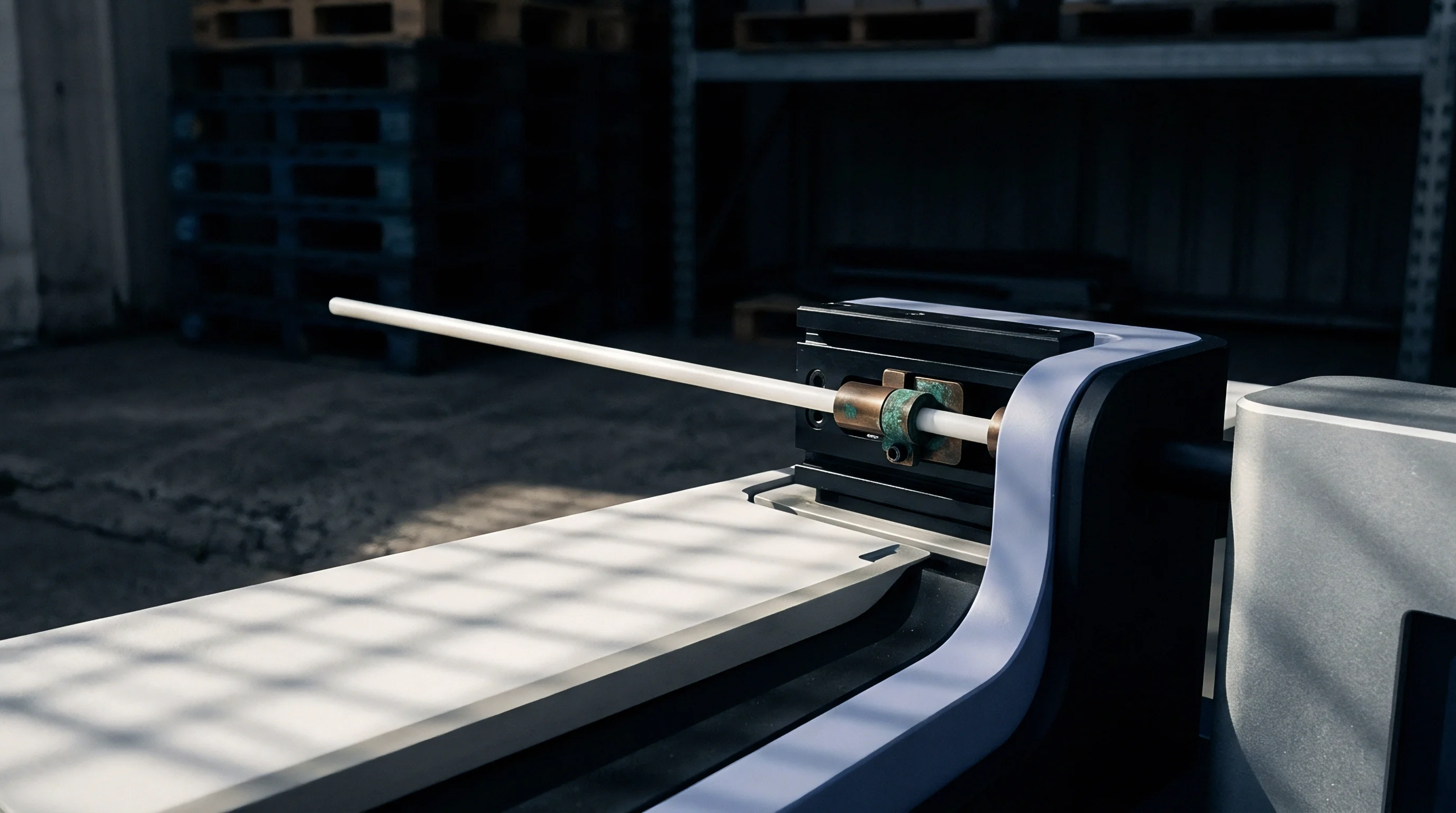
Mechanical accuracy of the tumble rig sets the baseline noise floor for sensor parameter estimation. An ideal fixture rotates the device under test through precise spatial angles without introducing mechanical wobble, shaft play, or thermal expansion shifts. Encoder errors and axis non-orthogonality within the positioning rig propagate directly into sensor misalignment matrices, distorting calculated non-orthogonality parameters.
Dimensional stability of multi-axis gimbal rings varies under changing ambient temperatures. Aluminum fixtures expand at approximately 23 micro-strains per kelvin, inducing angular tilt errors across mounting plates as laboratory conditions cycle. Stainless steel or Invar structures minimize thermal expansion distortion, maintaining angular indexing accuracy within sub-arcsecond tolerances during multi-hour calibration runs.
| Error Source | Physical Mechanism | Magnitude Range | Impacted Sensor Parameter | Mitigation Strategy |
|---|---|---|---|---|
| Encoder Angular Error | Optical disk eccentricity and grating line imperfections | 2 to 15 arcseconds | Cross-axis misalignment matrix | Dual-readout high-resolution optical encoders |
| Axis Non-Orthogonality | Machining and bearing alignment tolerances | 5 to 30 arcseconds | Sensor non-orthogonality parameters | Laser interferometer alignment and rig compensation |
| Gimbal Structural Deflection | Gravity vector induced strain on overhang arms | 0.01 to 0.05 millirad | Secondary axis bias shifts | FEA-optimized closed-frame gimbals |
| Thermal Frame Expansion | Differential thermal expansion of metal structural parts | 10 to 50 ppm/deg C | Scale factor temperature coefficients | Invar construction with temperature-controlled housing |
| Drive Motor Vibration | Bearing roughness and motor cogging forces | 0.5 to 3.0 milli-g RMS | Noise floor and residual error variance | Direct-drive brushless motors with static brake locking |
Rig mechanical degradation manifests through specific structural failure modes during extended production use:
- Gimbal bearing runout introduces parasitic angular motion during rotation steps, creating random vector magnitude perturbations across tumble positions.
- Drive shaft torsional windup causes orientation lag when switching rotation directions, inserting directional hysteresis errors into cross-axis calibration parameters.
- PCB mounting socket flexure warps the device substrate under gravitational load flips, blurring internal die strain with fixture structural bending.
- Thermal gradient development across direct-drive motor housings transfers heat to the DUT socket, causing uncontrolled bias shifts during static dwell periods.
Compliance with ISO/IEC 17025 Section 7.6 mandates complete measurement uncertainty budgets for automated sensor calibration rigs, explicitly requiring physical fixture orientation errors alongside sensor digital noise figures. Audits reject calibration certificates derived from rigs lacking verified optical encoder traceability records.

Proof
Validating calibrated parameter matrices requires post-optimization verification against independent orientation datasets. Re-running the original tumble dataset through optimized matrix transformations measures fitting efficacy, but fails to evaluate model generalization. Testing the sensor across uncalibrated intermediate spatial angles exposes residual mapping errors, over-fitting artifacts, and unmodeled non-linearities.
Sphere fitting verification calculates vector magnitude residual distributions across a dense 3D spatial rotation domain. Uncalibrated accelerometer outputs form a tilted, shifted ellipsoid in 3D field space. Applying optimized parameter matrices transforms raw data points onto a unit sphere centered at the origin.
The standard deviation of vector radius residuals directly indicates residual non-linearity and uncompensated noise.
Uncompensated thermal gradients inside the sensor cavity distort scale factor matrices faster than second-order optimization routines can resolve.
Evaluating parameter stability across operational boundaries requires a systematic verification procedure:
- Out-of-sample orientation evaluation subjects the calibrated sensor triad to 16 intermediate orientation angles not present in the optimization dataset.
- Residual magnitude distribution mapping plots vector magnitude errors against spatial orientation coordinates to locate localized mapping distortions.
- Allan variance analysis measures post-calibration bias stability across integration time scales ranging from 0.1 seconds to 10,000 seconds.
- Thermal chamber validation sweeps cycle ambient temperature across -40 to +85 degrees Celsius while running verification tumble sequences to confirm thermal model fit.
Operational verification following matrix estimation proceeds through this sequence:
- Mount the calibrated sensor module into an independent, optical-encoder-verified single-axis rotation tilt table.
- Apply continuous 360-degree pitch rotations at a constant rate of 10 degrees per second while recording converted sensor readings.
- Compute normalized spatial vector magnitudes for every sampled point across the full 360-degree rotation circle.
- Subtract the local scalar reference magnitude from calculated readings to generate a continuous error residual trace.
- Confirm that peak residual error bounds remain within three standard deviations of the sensor native broad-band noise floor.
Post-optimization, residual vector magnitude error variance should match the native thermal noise floor of the internal sensing element.

Throughput
Integrating non-linear tumble matrix calibration into high-volume sensor manufacturing demands balancing cycle time against accuracy goals. A 36-position tumble routine with 30-second thermal dwell periods consumes over 20 minutes per device, creating severe line bottlenecks. High-volume facilities address this by using multi-socket tumble trays inside environmental test chambers to calibrate hundreds of sensor ICs in parallel.
| Calibration Strategy | Cycle Time Per Tray (min) | Parameter Output Count | Residual Magnitude Error (milli-g) | Landed Unit Test Cost ($) |
|---|---|---|---|---|
| Single-Axis Static Flip | 2.5 | 6 (Linear Bias & Scale) | 12.5 | 0.15 |
| 12-Position Multi-Axis Tumble | 8.0 | 12 (Bias, Scale, Cross-Axis) | 2.1 | 0.48 |
| 24-Position Non-Linear Optim. | 18.5 | 21 (Non-Linear + g-Sensitivity) | 0.3 | 1.25 |
| 36-Pos. Full Thermal Matrix | 45.0 | 33 (Full Thermal & High-Order) | 0.08 | 3.10 |
Once optimization solvers complete parameter extraction, calculated float32 values are programmed directly into sensor module non-volatile EEPROM registers. Internal ASIC signal processing engines apply real-time compensation in hardware, outputting fully corrected physical vector readings over SPI or I2C bus interfaces.
Payback periods for automated calibration equipment depend directly on multi-socket tray density and gimbal indexing speed. Sourcing high-grade inertial sensors requires auditing the actual tumble matrix calibration setup to verify that high-order non-linear terms are calculated across full operating thermal bounds rather than generated through software extrapolation.