What Sensor Calibration Is and Why Readings Drift
Calibration maps sensor error against traceable standards, while drift stems from physical aging, mechanical strain, and environmental stress over time.

Reference
Transduction Physics and Transfer Function Definition
Every sensor is fundamentally a physical transducer converting a mechanical or environmental property into an electrical signal. In theory, that signal tracks the input stimulus with absolute fidelity through a simple mathematical formula ~ whether measuring voltage, current, capacitance, or frequency. In practice, real sensor outputs deviate from ideal models.
Take a piezoresistive silicon pressure die: mechanical strain alters the semiconductor’s band structure and shifts local resistivity. That shift responds not only to applied pressure but also to lattice temperature, dopant density variations across the silicon, and residual mechanical stress from packaging. Establishing the true input-output mapping requires systematic testing across the entire operating range.
Defining this mathematical relationship sits at the heart of sensor metrology. Instrument behavior is typically described by a transfer function, usually written as a polynomial expansion linking output voltage to the measured parameter. Zero-point offset is the output when no stimulus is present.
Span, or sensitivity, sets the function’s slope ~ the voltage change per unit of input change. Higher-order polynomial terms account for non-linearity, capturing how the response curves away from a straight line between zero and full scale. End-point non-linearity measures this departure relative to a line drawn directly between terminal calibration points, while best-fit straight line non-linearity compares it against an optimized linear regression.
Repeatability measures how consistently the transducer returns the same output when exposed to identical inputs in consecutive runs from the same direction.
Hysteresis complicates the transfer function further by making output dependent on the transducer element’s recent thermal or mechanical history. Loading a pressure transducer from zero up to full scale causes diaphragm strain to follow a specific deformation path. Upon unloading, microscopic internal friction, polymer relaxation in die-attach adhesives, and lattice micro-strains prevent the diaphragm from retracing that path in reverse.
The voltage difference recorded at a given pressure during depressurization is the hysteresis error. Quantifying zero offset, span sensitivity, non-linearity, and hysteresis establishes a transducer’s accuracy envelope under specific laboratory conditions.
- Primary reference standard verification against national metrology institutes ensures baseline measurement uncertainty remains documented prior to device exposure.
- Environmental test chamber stabilization holds ambient temperature within zero point one degrees Celsius and relative humidity within two percent.
- Multi-point stimulus application sweeps the full operating scale across at least five ascending and five descending test points to capture directional hysteresis.
- Uncertainty budget computation incorporates reference standard expanded uncertainty, test fixture thermal drift, and device digital resolution limits.
- Issuance of standard ISO 17025 measurement documentation records unadjusted raw outputs alongside calculated correction polynomials for system integration.
Evaluating a transducer requires separating its intrinsic noise floor from systematic sensor errors. Resolution is the smallest change in physical stimulus that yields a measurable output change ~ a limit set by thermal noise, ADC quantization, and amplifier flicker noise. A sensor with high resolution and tight precision can still suffer from substantial systematic offset.
Precision describes the statistical spread of repeated readings around their mean under stable conditions, while accuracy measures how close those readings come to the true value defined by an international standard. Precision comes from statistical variance; accuracy requires direct comparison against certified physical standards.

Distinction between Calibration Adjustment and Trim
Evaluating an instrument requires distinguishing formal metrological measurement from altering device settings. Measuring a sensor against a standard without modifying internal coefficients or signal processing constitutes calibration. What emerges from this process is documented evidence: raw readings, calculated corrections, and an uncertainty budget framing the test’s confidence level.
Calibration identifies systematic errors without touching hardware or firmware registers, though operating engineers sometimes mistake it for a repair, expecting a calibrated unit to return showing zero error.
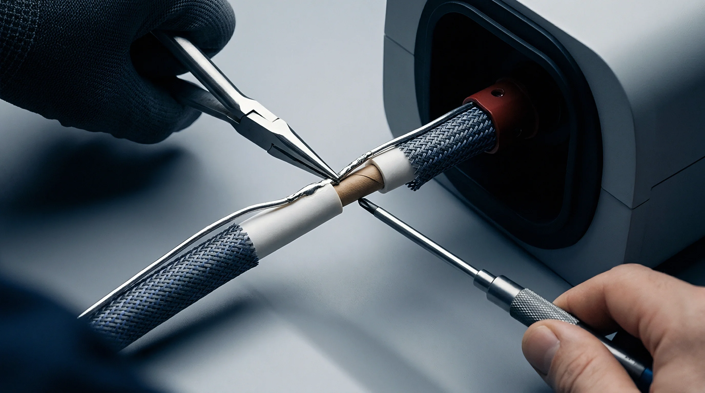
Modifying internal parameters to match reference readings constitutes zero-point trim or span adjustment. On digital sensors, this involves updating lookup tables in non-volatile flash memory or adjusting internal DAC registers. Analog sensors require physically turning potentiometers, laser-trimming resistor networks, or changing amplifier gain stages.
Zero trim shifts the transfer function vertically to eliminate offset; span trim adjusts the slope to correct gain errors across the full range. While adjustments change future device behavior, they permanently overwrite historical raw error profiles unless pre-adjustment calibration data was recorded first.
A calibration certificate without stated measurement uncertainty provides zero metrological value.
A basic two-point factory trim fixes linear offset and gain errors while leaving non-linear curvature untouched. If a piezoresistive sensor shows second- or third-order polynomial non-linearity from its diaphragm geometry, a two-point adjustment aligns output with the standard only at zero and full scale. Mid-scale readings retain residual non-linearity that can easily exceed the instrument’s basic accuracy rating.
High-precision designs rely instead on multi-point polynomial correction, using onboard microprocessors to store third- or fifth-order matrix profiles mapped across several stimulus levels and temperatures. Yet even digital compensation cannot undo dynamic micro-structural changes in transducer physics that occur after the matrix is programmed into memory.

Traceability Chains to National Standards
Linking a field sensor reading to an international unit definition requires an unbroken, documented sequence of comparisons called a metrological traceability chain. At the apex sit physical realizations of Système International base units maintained by national metrology institutes like NIST in the United States or PTB in Germany. Primary laboratory standards sit just below them, kept under strict environmental controls to minimize long-term drift.
Secondary and working standards are verified against primary references at scheduled intervals, accumulating progressively larger uncertainty budgets further down the chain.
Every step down the traceability chain introduces its own uncertainty. When a working standard calibrates a field pressure transmitter, the field unit’s overall uncertainty pools uncertainties from the national standard, the primary calibration step, the working standard, lab environmental noise, and the instrument’s digital resolution. Standard metrology practice calculates combined standard uncertainty as the root-sum-square of all individual variance terms, applying a coverage factor—typically two—to establish a ninety-five percent confidence interval.
Without a fully documented traceability chain supported by unbroken certificates and explicit uncertainty budgets, accuracy claims remain simple commercial assertions.
Digitizing signals directly at the sensing die does not eliminate drift, as the underlying physical transducer still degrades over time.


Strain

Mechanical Creep and Package Stress Transference
Drift is the slow, systematic shift in sensor transfer function parameters over time under constant physical conditions. While environmental noise causes brief statistical jitter around a mean reading, drift permanently pulls baseline output and sensitivity away from calibrated values. In solid-state and MEMS sensors, this long-term drift stems largely from mechanical strain relaxation inside the assembly.
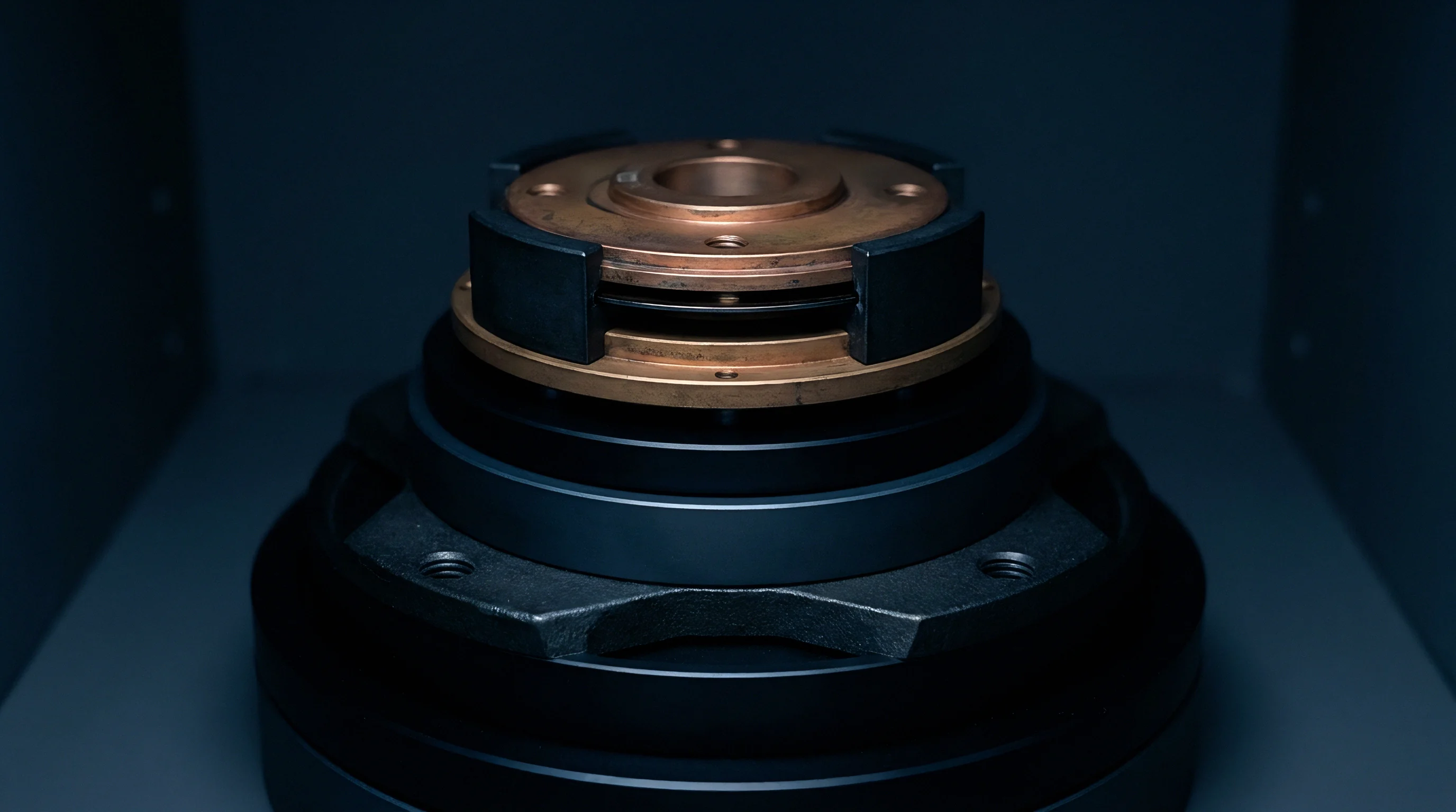
Sensor dies are bonded to ceramic substrates or metal headers using epoxies, glass frits, or metallic eutectic preforms ~ materials that each carry a distinct Coefficient of Thermal Expansion.
As temperatures cycle, mismatched thermal expansion rates create severe shear stress across bonding interfaces. A silicon die with an expansion coefficient of two point six parts per million per degree Celsius bonded to a copper leadframe at sixteen point five parts per million, for example, experiences heavy compressive stress as it cools from curing temperatures down to ambient. Over months of operation, internal micro-strains in organic epoxy undergo viscoelastic creep.
As that bond slowly relaxes, residual pre-stress transferred to the silicon diaphragm shifts continuously, altering the die’s baseline piezoresistive state and driving zero-point drift regardless of applied pressure.
This mechanical relaxation follows logarithmic decay, progressing fastest immediately after assembly and packaging. Over long operational periods, thermal cycling accelerates micro-cracking along the die-attach interface, causing non-linear baseline wander. High-precision pressure sensors using hard eutectic die-attach materials like gold-tin exhibit far less long-term creep than those built with soft silicone or epoxy adhesives, though hard solders transfer higher initial packaging stress directly to the active element.
Lattice Imperfections and Substrate Relaxation
Solid-state transducer elements undergo atomic-level degradation within their crystal structures that alters electrical behavior over time. In piezoresistive strain gauges and thin-film platinum RTDs, continuous operating stress and high temperatures trigger point defects, vacancy migration, and dislocation climb in the lattice. On thin-film platinum elements deposited on ceramic substrates, oxygen diffuses into grain boundaries at temperatures above two hundred degrees Celsius.
This interstitial oxidation shortens the electron mean free path, pushing ice-point resistance higher while lowering the temperature coefficient of resistance.
| Sensing Modality | Dominant Drift Mechanism | Typical Annual Wander | Primary Driver | Structural Mitigation |
|---|---|---|---|---|
| Piezoresistive Strain Gauge | Die-attach organic polymer creep | 0.15% to 0.40% Full Scale | Thermal cycling stress | Eutectic gold-tin die bonding |
| NDIR Optical Gas Sensor | IR emitter source intensity decay | 1.50% to 3.00% Full Scale | Filament evaporation & mirror fouling | Dual-beam reference channel ratioing |
| MEMS Capacitive Accelerometer | Charge trapping in dielectric isolation | 2.00 to 8.00 mg | High electrostatic bias voltage | Polysilicon shield layers and AC bias |
| Platinum Thin-Film RTD | Grain boundary oxidation & sub-layer diffusion | 0.05 to 0.15 degrees C | Continuous high temperature | Hermetic glass passivation capping |
In capacitive MEMS devices such as accelerometers and differential pressure sensors, structural drift is often caused by charge trapping in dielectric isolation layers. High electrostatic bias voltages across tiny air gaps push charges into silicon dioxide or silicon nitride passivation coatings. These trapped surface charges create parasitic electrostatic forces acting on the suspended proof mass, mimicking real acceleration or pressure shifts and permanently shifting the capacitive zero offset.
Because charge trapping kinetics depend on humidity ingress, bias polarity, and operating hours, the resulting drift profiles are complex and cannot be modeled by simple linear extrapolation.
Sensors subjected to thermal cycling drift faster than sensors operating continuously at elevated temperature.
Metal foil strain gauges attached to structural members accumulate mechanical hysteresis under cyclic fatigue loading. Microscopic plastic deformation along slip planes work-hardens the base metal. Its gauge factor ~ the resistance-to-strain ratio ~ shifts as micro-cracks grow through the constantan or karma alloy matrix.
Moisture absorption by the epoxy backing aggravates the issue, lowering electrical isolation between the foil element and the grounded specimen and creating parallel leakage paths that show up as false downward drift.
Relying on initial factory specifications across a three-year lifecycle allows unmonitored sensor drift to cause out-of-spec product returns, warranty costs, and hidden process errors.


Environment
What Triggers Accelerated Drift in Sealed MEMS Assemblies?
Moisture entering protective sensor housings represents one of the main environmental drivers of uncalibrated drift. Standard plastic packages, such as epoxy transfer-molded SOIC ICs and polycarbonate enclosures, have measurable Water Vapor Transmission Rates. Over months, water molecules diffuse through polymer housing walls and seal joints, elevating internal cavity humidity.
Once inside, moisture acts directly on micro-machined mechanical structures, high-impedance amplifier nodes, and sensitive sensing films.
In capacitive MEMS structures, water vapor alters the dielectric permittivity of the internal cavity. Air sits near a dielectric constant of one point zero, whereas liquid water approaches eighty at room temperature. Microscopic condensation or thin water layers on capacitive comb-finger electrodes increase inter-electrode capacitance, pulling the zero offset far outside factory tolerances.
Moisture ingress also causes stiction in MEMS accelerometers: capillary forces overcome the restoring force of silicon suspension springs, pinning moving proof masses permanently against mechanical stops.
High humidity accelerates surface dendrite growth and galvanic corrosion whenever ionic contaminants sit on the substrate. Trace chlorine or sulfur left from soldering flux dissolves in moisture films, forming conductive liquid bridges between adjacent high-impedance traces. These leakage paths shift op-amp bias currents and distort analog signal conditioning before digitizing.
High-impedance circuits ~ like glass-electrode pH sensors and tera-ohm piezoelectric charge amplifiers ~ experience severe baseline drift whenever surface insulation resistance drops from moisture absorption.
Moisture Ingress and Polymer Matrix Swelling
Humidity sensors using hygroscopic polymer films suffer structural degradation that distorts calibration curves over time. These sensors track capacitance or impedance shifts as water molecules enter a polyimide or polymer matrix. Ongoing exposure to volatile organic compounds, industrial solvents, or airborne plasticizers contaminates the polymer layer; organic molecules occupy binding sites intended for water, permanently lowering sensitivity and causing negative span drift.
- Die Bond Delamination relaxes mechanical boundary constraints on piezoresistive diaphragms, inducing unpredictable zero-point wander and thermal hysteresis shifts.
- Polymer Plasticization alters sorption kinetics within capacitive relative humidity elements, shifting baseline sensitivity and broadening measurement response time.
- Contaminant Deposit Layering coats optical windows in NDIR sensing chambers, attenuating light intensity and mimicking gas concentration increases.
- Electrode Surface Poisoning deactivates catalytic reaction sites in electrochemical gas sensors, causing steep loss of span sensitivity across operational cycles.
Combining high ambient humidity with elevated operating temperatures causes polymer plasticization. Water molecules weaken intermolecular hydrogen bonds in the polyimide chain, lowering the film’s glass transition temperature. The resulting structural softening swells the sensing layer and alters mechanical stress on the underlying silicon.
This swelling creates baseline zero drift and worsens hysteresis, since the plasticized polymer holds onto absorbed moisture longer during drying cycles than it does when wetting.
Oxidation Kinetics and Surface Contamination
Chemical reactions between sensing elements and surrounding gases gradually shift baseline resistance and chemical response curves. Electrochemical sensors for toxic gas detection use aqueous electrolytes and catalytic gas diffusion electrodes. As target gases react at the working electrode, solvent evaporates through the porous hydrophobic membrane into dry air.
Electrolyte loss increases internal cell resistance, reducing sensitivity and driving zero drift. Exposure to gas levels above full scale can poison electrode surfaces or saturate catalytic sites, permanently changing the calibration slope.
Relative humidity shifts above 85 percent at 60 degrees Celsius accelerate thin-film resistor degradation by a factor of four compared to ambient laboratory storage.
Optical sensors like non-dispersive infrared (NDIR) gas detectors drift as light sources degrade and optical paths become contaminated. NDIR sensors measure infrared absorption across target wavelengths based on the Beer-Lambert law. Over continuous use, incandescent micro-lamps experience tungsten filament evaporation, gradually dimming output intensity.
At the same time, dust, oil films, or organic outgassing settle on gold-plated reflection tubes and reduce reflectivity. In a single-beam detector, light loss from mirror fouling looks identical to absorption by target gas, creating positive zero drift. High-precision optical sensors add a dual-wavelength reference channel to compensate for broad light source decay and uniform fouling, though uneven contamination across channel filters can still cause residual drift.
How material formulators will eliminate moisture-induced hysteresis in high-temperature silicone encapsulation compounds remains an open question in sensor packaging research.


Budget

Combined Measurement Uncertainty Calculations
Quantifying calibration quality requires a comprehensive measurement uncertainty budget following the Joint Committee for Guides in Metrology Guide to the Expression of Uncertainty in Measurement. An accuracy claim on a commercial datasheet remains an unverified performance target unless accompanied by an expanded uncertainty figure calculated under defined statistical conditions. Evaluating total uncertainty means sorting error sources into Type A evaluations (from statistical analysis of repeated observations) and Type B evaluations (from scientific judgment, calibration certificates, vendor specs, and thermal drift models).
Building an uncertainty budget starts with a measurement equation defining the output as a function of input variables, reference standards, environmental influences, and resolution limits. Each input carries a standard uncertainty. For Type B components with a normal distribution, standard uncertainty is the quoted expanded uncertainty divided by the coverage factor (usually two).
For rectangular uniform distributions ~ like digital display resolution limits or thermal chamber control bands ~ standard uncertainty is the half-width of the tolerance interval divided by the square root of three. Triangular distributions, used when values cluster near the center of a tolerance band, divide by the square root of six.
| Uncertainty Component | Standard Uncertainty (kPa) | Probability Distribution | Sensitivity Coefficient | Uncertainty Contribution (kPa) |
|---|---|---|---|---|
| Primary Reference Standard | 0.0120 | Normal (k=2) | 1.00 | 0.0120 |
| Thermal Chamber Gradient | 0.0250 | Rectangular | 1.00 | 0.0144 |
| Sensor Non-Repeatability | 0.0180 | Normal (k=1) | 1.00 | 0.0180 |
| ADC Quantization Resolution | 0.0050 | Rectangular | 1.00 | 0.0029 |
| Power Supply Voltage Variation | 0.0080 | Rectangular | 0.50 | 0.0023 |
| Combined Standard Uncertainty: 0.0264 kPa | Expanded Uncertainty (k=2, 95% Confidence): 0.0528 kPa | ||||
Combining individual standard uncertainties requires multiplying each term by its partial derivative sensitivity coefficient, which measures output change per unit change of that input. If input variables are statistically independent, combined standard uncertainty is the root-sum-square of the individual uncertainty contributions. When components correlate ~ such as simultaneous thermal drift in reference standards and amplifiers driven by room temperature shifts ~ covariance terms must be calculated and added to the sum.
The effective degrees of freedom are calculated using the Welch-Satterthwaite equation to select the correct coverage factor for expanded uncertainty at the target confidence level.
Guardbanding Strategies for High-Yield Acceptance
Verifying product compliance during incoming inspection or manufacturing calibration requires managing decision risk from measurement uncertainty. When a measured value sits near a specification limit, uncertainty creates false acceptance or false rejection risks. A false acceptance happens when an out-of-spec sensor passes inspection because test error shifts the reading inside the limits.
Conversely, a false rejection hurts manufacturing yield by scrapping good hardware whose reading was pushed outside tolerance by test rig uncertainty.
Mitigating consumer risk requires guardbanding protocols aligned with ISO 14253-1 and ANSI/NCSL Z540.3. Guardbanding shrinks the acceptance zone by pulling specification limits inward by a distance proportional to the calibration rig’s expanded uncertainty. A 1:1 guardband subtracts one times the expanded uncertainty from the upper limit and adds it to the lower limit.
Sensors measuring within this narrowed band ensure the probability of false acceptance stays below target risk thresholds ~ typically under two percent for ISO 17025 accredited labs.
ISO 17025 clause 7.8.4 mandates that recalibration certificates state coverage factors and expanded uncertainty, transferring legal liability for uncalibrated drift directly to the instrument operator.
Strict guardbanding raises lot rejection rates if test rig uncertainty is large relative to sensor tolerances. Maintaining high yield while keeping false acceptance low depends on controlling the Test Uncertainty Ratio ~ the sensor’s tolerance band divided by the expanded uncertainty of the calibration system. A minimum Test Uncertainty Ratio of 4:1 keeps acceptance zones from shrinking too drastically, preserving yield while keeping out-of-spec hardware out of the field.

Commercial Cost of Calibration Intervals
Setting calibration intervals is a balancing act between the financial risk of unmonitored drift and the direct cost of recalibration downtime and lab fees. Running a sensor continuously without recalibration risks silent process drift ~ where unverified measurements lower product yield, waste energy, or trigger compliance failures. On the other hand, setting overly aggressive recalibration cycles inflates maintenance labor, consumes spare parts, and disrupts production without delivering meaningful gains in accuracy.
Dynamic interval strategies use historical drift trends to optimize service schedules under ISO 10012 guidelines. Standard calendar-based schedules assign fixed annual or semi-annual dates regardless of operating hours or thermal exposure. That static method often fails when sensors face severe thermal cycling or humidity, where drift runs far ahead of lab baselines.
A better approach relies on drift-rate trend analysis: tracking successive calibration records by serial number lets engineers calculate mean time to out-of-tolerance failure and adjust service intervals to catch drifting units before they cross guardband limits.
Including ISO 10012 section 7.1 in procurement contracts requires suppliers to provide verified historical drift data, shifting the burden of proving stability from the buyer to the manufacturer.
Protocol

Bench Verification Workflows and Environmental Control
Valid calibration routines for high-accuracy sensors require strict control over bench environments and workflows. Lab conditions must stay within tight tolerances so thermal gradients, barometric shifts, and humidity swings do not distort test data. Standard metrology labs hold ambient temperature at twenty degrees Celsius plus or minus zero point five degrees, keeping relative humidity under fifty percent to prevent surface condensation on high-impedance electrical connections.
Before recording verification data, sensors and reference standards need a thermal soak period inside the controlled lab space. A stainless steel pressure transducer or heavy optical housing brought in from an unheated warehouse takes hours to reach internal thermal equilibrium. Taking readings while internal temperature gradients exist generates transient thermal EMF across solder joints and causes differential thermal expansion between sensing diaphragms and supports, producing substantial zero-offset errors.
| Operational Dimension | Calibration | Adjustment | Trim |
|---|---|---|---|
| Primary Purpose | Quantify error and uncertainty | Modify system output slope/offset | Fine-tune hardware baseline |
| Hardware Modification | None performed | Software EEPROM table write | Potentiometer or laser resistor edit |
| Historical Data Preservation | Preserves raw error record | Erases unadjusted baseline output | Erases original analog output curve |
| Traceability Requirement | Mandatory ISO 17025 link | Optional operational step | Factory internal procedure |
| Execution Frequency | Periodic service interval | Performed post-calibration if needed | Performed during manufacturing build |
Standard verification workflows use structured multi-point profiles to isolate specific error sources. A basic three-point calibration checks zero, fifty percent, and full-scale output to verify baseline gain and offset. High-precision jobs use an eleven-point up-and-down cycle, taking readings at ten percent scale increments from zero to one hundred percent and back.
Sweeping up and down through stimulus levels captures peak non-linearity, terminal span errors, and total mechanical hysteresis. Automated calibration benches combine programmable pressure controllers, precision oil baths, and digital multimeters managed by test scripts, removing operator bias and ensuring repeatability across test runs.

Field Calibration Standards and Automated Trim
Field verification brings challenges not encountered on a lab bench. Accuracy must be verified in operating environments where ambient temperature shifts, structural vibration, and dirty process fittings threaten measurement validity. Portable field calibrators must carry active ISO 17025 certificates showing at least a 4:1 Test Uncertainty Ratio over the target instrument, using internal temperature compensation to maintain accuracy across variable field conditions.
- Operating Temperature Excursion History determines whether thermal hysteresis has permanently shifted baseline polynomial compensation coefficients.
- Measurement Risk Classification dictates whether a 1:1 guardband or a 2:1 guardband must be applied to incoming verification acceptance limits.
- Historical Drift Rate Extrapolation indicates whether the scheduled recalibration interval should be shortened due to accelerated zero wander.
- Regulatory Compliance Requirements enforce mandatory fixed-interval laboratory recalibration regardless of observed field performance stability.
Executing an automated field trim updates digital compensation registers without pulling the sensor from process piping. Smart HART, Modbus, or IO-Link sensors let field calibrators send zero and span commands directly to the microcontroller. The routine reads raw ADC values, compares them against reference standard inputs, calculates new offset and gain factors, and writes them to onboard non-volatile memory.
Modern field calibrators log pre-adjustment as-found values alongside post-adjustment as-left values, uploading the entire record to enterprise asset management software to maintain historical traceability for audits.
When a sensor output drifts past half its allowable tolerance, scheduling recalibration prevents unexpected out-of-tolerance failures.