Quantifying Early Zero Drift in Precision Strain Gages
Quantifying early zero drift requires isolating initial thermal self-heating transients from viscoelastic polymer stress relaxation using standardized 168-hour bench burn-in protocols.

Foil
Immediately after structural mounting and power-up, precision strain gage installations display non-linear output drift. This early zero drift plays out over the first minutes, hours, and days of operation, masking real mechanical strain and skewing low-level tare values. The underlying physical drivers stem from the microstructural mechanics of the sensor matrix itself.
Bonded metallic resistance gages use a thin conductive grid etched from alloys like constantan or nickel-chromium, encapsulated in a polymeric carrier substrate. When an adhesive bonds this assembly to a test article, the entire composite system is trapped in a non-equilibrium mechanical and chemical state.
Polymer carriers and organic bonding agents have viscoelastic properties that drive continuous stress redistribution long after installation. Factory processes introduce residual stresses into polyimide or epoxy-phenolic backing films during solvent evaporation and thermal curing. Once clamped down, the adhesive layer adds its own cure shrinkage stresses across the bond line.
As these organic matrices slowly relax toward thermodynamic equilibrium, their dimensions shift on a micro-inch scale. Because the conductive foil grid is bonded right to the carrier, those dimensional changes impart parasitic mechanical strain onto the grid elements ~ altering the baseline electrical resistance of the Wheatstone bridge without any change in applied load.
Polymer Backing Viscoelasticity and Stress Relaxation
Polymeric carrier materials undergo primary creep and volumetric relaxation under residual mechanical stress. Polyimide films experience time-dependent deformation under the continuous low-level shear generated by the bond. Epoxy-phenolic carriers offer higher dimensional stability than polyimide, but remain vulnerable to localized strain relief along their molecular chains.
Polymeric stress relaxation follows an inverse exponential rate, moving quickly over the first 10 hours before settling into a steady background rate after roughly 168 hours.
Polymer backings undergo creep under continuous load.
Adhesive choice governs both the scale and duration of this initial relaxation phase. Room-temperature curing cyanoacrylates allow quick turnaround times, but produce high internal strain gradients. These fast-curing matrices keep cross-linking and outgassing through the first 48 hours in the field, causing noticeable zero-point wander.
Heat-cured epoxy systems undergo high-temperature polymerization that minimizes residual room-temperature cross-linking. Even so, thermal expansion mismatches between the curing fixture, gage carrier, and structural alloy leave locked-in shear stresses across the interface upon cooling. As these thermal stresses relax, they create a steady positive or negative zero drift depending on how the expansion coefficients align.
A constant excitation of 5 volts across a 350-ohm polyimide strain gage mounted on aluminum produces a thermal zero shift of 14 microstrain during the initial 45 minutes of energization.
Grid Alloy Lattice Stability and Annealing Kinetics
Metallic strain-sensing foils undergo atomic lattice realignment during cold-rolling and chemical etching. Constantan alloy ~ 55 percent copper and 45 percent nickel ~ is processed to achieve a near-zero temperature coefficient of resistance at ambient conditions. Cold rolling leaves dislocation densities in the grain structure that modify local resistivity.
While thermal annealing during sensor production relieves bulk lattice strain, residual dislocations remain concentrated near the etched grid edges.
Handling during fabrication hardens the resistive foil.
Once electrical excitation energizes the gage, Joule heating raises the grid temperature above the surrounding substrate baseline. This local heating drives low-level atomic diffusion, letting residual lattice dislocations migrate toward grain boundaries. The resulting microstructural annealing reduces the foil’s bulk electrical resistance during early operation, shifting nominal resistance and producing an uncommanded zero offset across the Wheatstone bridge.
Nickel-chromium alloys offer better lattice stability than constantan, but undergo short-term order-disorder phase transitions between 50 and 120 degrees Celsius that shift baseline resistance during initial thermal cycles.
The grid foil relaxes mechanically after bonding.
The mechanisms driving early zero drift operate simultaneously across the backing film, adhesive layer, and metallic grid. The net drift trajectory is the algebraic sum of backing relaxation, adhesive shrinkage, and foil lattice annealing. When these forces act in opposing directions, partial cancellation masks the underlying instability.
When they align, zero wander quickly exceeds the annual calibration limits of high-precision load cells and structural monitoring arrays.
- Adhesive Cure Contraction volumetric shrinkage of organic bonding agents creates localized compressive strain across the foil grid during initial post-cure cross-linking.
- Polymer Backing Creep time-dependent shear deformation within polyimide or epoxy carrier films transfers residual manufacturing stresses directly into the sensing element.
- Grid Defect Recovery thermal activation from bridge excitation drives dislocation migration in cold-worked foil alloys, permanently altering baseline electrical resistance.
- Interfacial Shear Relaxation stress dissipation along the adhesive-substrate boundary alters mechanical load transfer efficiency prior to reaching thermodynamic equilibrium.
Ignoring early zero drift metrics during installation risks mistaking initial stress relaxation for structural settling or material yield in the test article, invalidating baseline tare calibrations over the first week of testing.

Bench
Isolating early zero drift requires lab instrumentation capable of separating mechanical sensor drift from thermal transients, lead wire resistance variations, and digitizer noise. Standard factory bench setups routinely miss true drift because room temperature fluctuations obscure microvolt-level changes in bridge balance. A proper qualification test places the mounted or unmounted transducer inside an environmentally controlled chamber held within tight thermal limits.
Excitation voltage is a key variable during zero-drift testing. Higher voltages boost signal-to-noise ratios by increasing microvolt output per microstrain, but also drive up self-heating inside the foil grid. For example, powering a 350-ohm gage at 10 volts causes the grid to dissipate roughly 286 milliwatts of thermal energy.
On substrates with low thermal conductivity, such as carbon fiber composites or titanium, this power dissipation raises grid temperature several degrees Celsius above ambient air. The resulting expansion and resistance shift register as early zero drift until thermal equilibrium forms across the grid, adhesive, and substrate.
Higher excitation voltage drives internal self-heating.
Thermal Stabilization Procedures and Excitation Management
Quantifying mechanical drift requires thermal equilibrium across the entire measurement loop before logging baseline data. Standard protocol calls for placing the sample inside a chamber held at 23.0 degrees Celsius with spatial stability within 0.1 kelvin. The specimen must soak unenergized for at least four hours to purge ambient thermal gradients across the substrate and lead wires.
Current-induced heating alters bridge balance.
Bridge excitation should come from regulated, low-noise lab power supplies using remote sensing at the gage terminals. When bridge voltage is first applied, an initial transient drift appears while self-heating warms the grid and adjacent adhesive. This thermal stabilization window typically lasts between 5 and 45 minutes, depending on substrate thermal mass and geometry.
Readings taken during this period reflect heat transfer dynamics rather than structural instability. Distinguishing thermal settling from true mechanical drift requires tracking substrate surface temperature using precision reference thermocouples or resistance thermometers placed right next to the installation.
ISO/IEC 17025 laboratory accreditation standards invalidate zero-point reference measurements taken before sensor thermal equilibrium reaches 0.05 kelvin per hour.
Bridge Balancing and Parasitic EMF Suppression
Parasitic thermoelectric voltages introduce notable errors during zero-drift evaluations. Thermal electromotive forces develop wherever dissimilar metals join across a temperature gradient. Solder joints linking copper lead wires to constantan or nickel-chromium gage tabs generate microvolt potential differences if thermal gradients cross the terminal pad area.
Under direct-current excitation, these parasitic voltages add directly to the Wheatstone bridge unbalance signal, mimicking zero drift as ambient temperatures fluctuate or internal heat dissipates.
Thermal gradients across joints skew bridge outputs.
Suppressing parasitic thermal voltages requires offset-compensated direct-current excitation or alternating-current carrier amplifier systems. Offset compensation measures bridge output in the unexcited state right before applying excitation pulses, subtracting the passive thermoelectric offset from the active signal. Pulsed direct-current excitation cuts total heat dissipation in the grid by reducing duty cycles to five percent or less, keeping self-heating low while preserving signal amplitude.
Alternating-current carrier systems modulate excitation at frequencies between 225 hertz and 5 kilohertz, filtering out static and low-frequency DC thermal voltages entirely.
| Excitation Mode | Thermal Dissipation (mW) | Equilibrium Time (min) | Thermal EMF Susceptibility | Zero Measurement Uncertainty (μm/m) |
|---|---|---|---|---|
| Continuous DC (10V, 350Ω) | 285.7 | 35 to 50 | High | ± 4.2 |
| Continuous DC (3V, 350Ω) | 25.7 | 8 to 15 | Moderate | ± 1.8 |
| Pulsed DC (10V, 5% Duty) | 14.3 | 2 to 5 | Low | ± 0.6 |
| AC Carrier (5V RMS, 4.8 kHz) | 71.4 | 12 to 20 | Zero (Filtered) | ± 0.4 |
Running a zero-drift benchmark follows a sequential isolation routine to maintain data integrity across multi-day test runs:
- Mount the strain sensor to a stress-free zero-expansion Invar 36 reference block inside a temperature-controlled chamber maintained at 23.0 degrees Celsius.
- Connect the half-bridge or full-bridge leads to a calibrated 24-bit strain gage digitizer using a four-wire Kelvin sense configuration.
- Apply the rated bridge excitation voltage and log the zero-point voltage output at one-second intervals for the initial 120 minutes.
- Subtract the calculated self-heating thermal transient response from the raw output curve to yield the net mechanical zero drift.
- Continue logging zero-point data at 60-second intervals under continuous environmental control for 168 hours to establish long-term decay slope coefficients.
Early zero changes are frequently assigned to user soldering techniques or substrate thermal expansion rather than residual manufacturing stress relief within commercial gage backings.

Decay
Modelling early zero drift mathematically requires logarithmic and multi-exponential decay functions to separate transient stabilization from long-term sensor degradation. Bench testing shows that early drift does not progress linearly over time. Instead, drift rates peak immediately after installation and power-up, decaying monotonically toward a constant asymptotic slope over extended service.
Static offsets follow a logarithmic decay curve.
The classic model for strain gage zero drift uses a logarithmic time function to describe post-bonding stress relaxation. Total zero shift at time t, expressed in microstrain, follows the relation:
S(t) = S_0 + A ln(1 + t / tau)
where S_0 represents the initial electrical offset upon energization, A is the logarithmic drift amplitude coefficient, t is elapsed time in hours, and tau is the characteristic relaxation time constant of the polymer matrix. Values for A and tau come from non-linear least-squares regression applied to bench data recorded during the first 48 hours of continuous operation.

Why Does Logarithmic Time Modeling Underestimate Late Wander?
Logarithmic decay functions accurately track primary viscoelastic stress relaxation during early operational hours. Pure logarithmic models, however, assume a continually diminishing drift rate that ignores secondary degradation like moisture diffusion and adhesive oxidation. Beyond 500 hours, physical drift curves bend upward from logarithmic predictions into a steady linear background drift.
Moisture absorption causes expansion in epoxy matrices.
Resolving this discrepancy requires a hybrid mathematical formulation combining short-term exponential terms with a linear long-term aging term:
S(t) = S_0 + B (1 – exp(-t / tau_1)) + C (1 – exp(-t / tau_2)) + K_drift t
Here, B and C represent short- and medium-term stress relief amplitudes, while tau_1 and tau_2 correspond to the quick thermal self-heating time constant (typically 0.1 to 0.5 hours) and the polymer cure time constant (typically 12 to 36 hours). The coefficient K_drift captures linear long-term drift in microstrain per thousand hours. Isolating these parameters allows projection of 8760-hour annual stability from a standard 168-hour laboratory burn-in.
Initial drift rates measured over hours reflect polymeric cure stresses, whereas drift measured over months indicates moisture ingress or metallic grid lattice relaxation.
Uncertainty propagation across these model coefficients limits long-term prediction accuracy. Small errors in fitting the initial 12-hour drift slope lead to wide divergence when extrapolating out over years of service. Calculating expanded measurement uncertainty requires accounting for variance in chamber temperature, bridge voltage drift, digitizer gain stability, and regression residual errors.
| Substrate / Adhesive Combination | Test Condition (Temp / RH) | 24-Hour Drift (μm/m) | 168-Hour Drift (μm/m) | Logarithmic Amplitude (A) | Time Constant tau (hours) |
|---|---|---|---|---|---|
| Polyimide Backing / Cyanoacrylate | 23°C / 50% RH | + 18.5 | + 26.2 | 4.12 | 0.85 |
| Polyimide Backing / Heat-Cured Epoxy | 23°C / 50% RH | – 3.2 | – 4.8 | 0.78 | 2.10 |
| Epoxy-Phenolic / Heat-Cured Epoxy | 23°C / 50% RH | – 1.1 | – 1.6 | 0.24 | 3.45 |
| Polyimide Backing / Heat-Cured Epoxy | 70°C / 85% RH | + 42.0 | + 89.4 | 14.80 | 0.45 |
| Epoxy-Phenolic / Heat-Cured Epoxy | 70°C / 85% RH | + 12.4 | + 28.1 | 4.35 | 1.20 |
| Data normalized for 350-ohm gages on 2024-T4 aluminum reference blocks with 5V DC excitation. Total measurement expanded uncertainty is ± 0.8 μm/m (k=2). | |||||
Determining the multi-variable cross-coupling threshold where environmental humidity permanently alters the short-term viscoelastic relaxation time constant remains critical for high-temperature ceramic strain gage adhesives.
Clamp
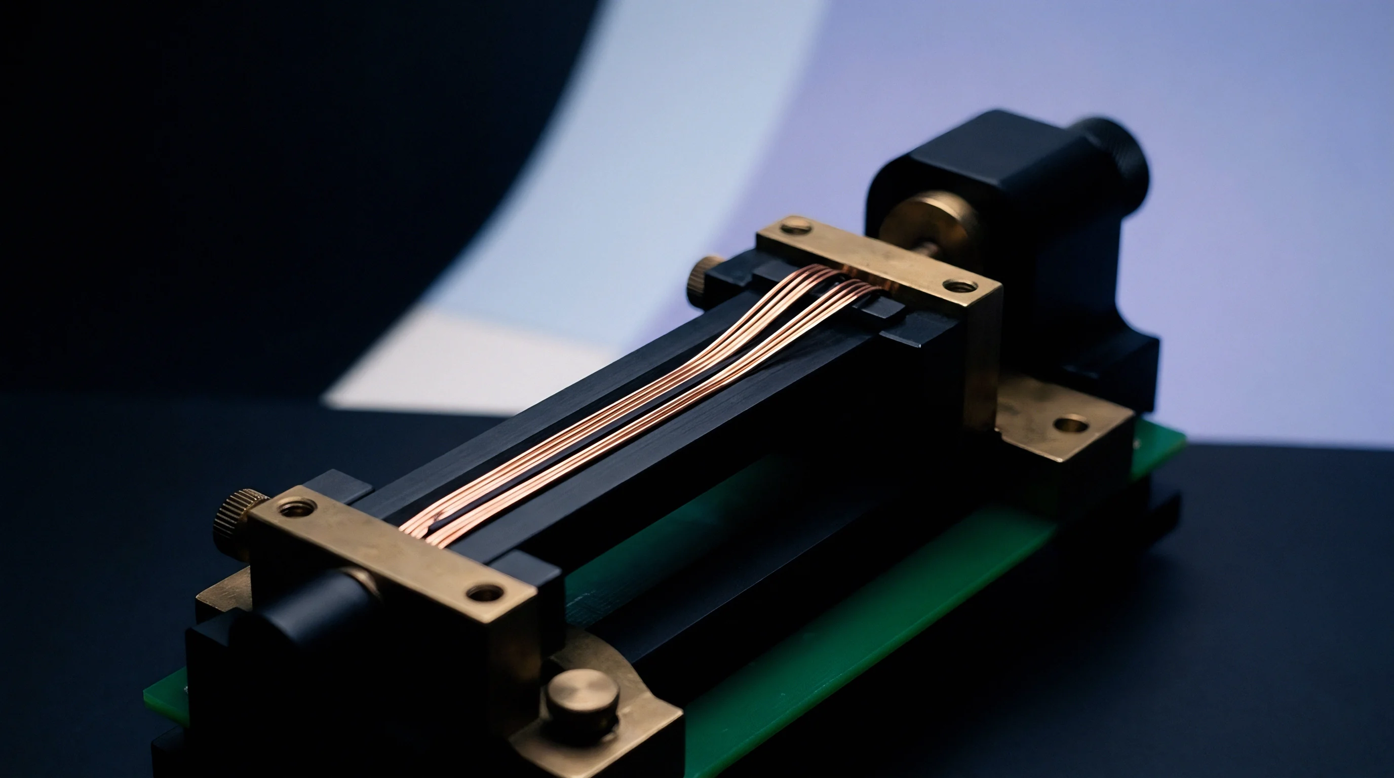
Mechanical installation dynamics and environmental boundary conditions directly dictate the magnitude of early zero wander in field-deployed strain gages. Clamping pressure applied during curing sets the thickness and uniformity of the bond line. Inconsistent clamping force across the active area leaves local stress concentrations and variable adhesive pockets.
Thicker bond lines increase total viscoelastic volume, raising absolute cure shrinkage strain and extending early drift.
Optimal clamping protocols specify uniform spring-loaded or pneumatic pressure between 0.10 and 0.25 megapascals during cure. Insufficient pressure traps air voids in the adhesive layer, creating localized compliance zones that distort strain transfer from the structure to the grid. Excess pressure starves the joint of adhesive, risking microscopic grid-to-substrate shorts or micro-cracking of the carrier film.
Both extremes elevate early zero drift by destabilizing the interfacial shear stress profile.

Bonding Pressure Distribution and Interfacial Shear
Interfacial shear stress transfer between the test structure and gage matrix determines the mechanical fidelity of the installation. If a structural member undergoes cyclic loading immediately after bonding, incomplete cross-linking causes interfacial mechanical hysteresis. Microscopic slip along the interface prevents full strain recovery when load is released, manifesting as a permanent zero-point shift.
Incompletely cured adhesive shifts zero output.
Allowing a mechanical resting period before testing reduces post-bonding zero instability. Curing schedules must also account for substrate heat-sink effects: thick metallic sections draw heat away during thermal cure cycles, preventing the adhesive from reaching target cross-linking temperatures. Incomplete thermal curing leaves low-molecular-weight oligomers in the polymer matrix, doubling early viscoelastic drift rates in early field service.
Encapsulant moisture absorption alters bridge symmetry by introducing asymmetric parasitic shunt resistances across neighboring gage arms.

Moisture Ingress and Parasitic Shunt Resistance Dynamics
Atmospheric humidity is a major driver of early zero drift in unsealed or poorly encapsulated strain gage installations. Polyimide backing films and epoxy adhesives are hydrophilic, absorbing moisture until reaching equilibrium. Water uptake expands the polymer matrix volume, producing swelling strain that stretches the bonded foil grid.
This swelling shows up as a positive zero drift that can exceed 100 microstrain under high relative humidity.
Moisture also introduces parasitic shunt paths parallel to the Wheatstone bridge arms. If condensed water vapor drops insulation resistance between the grid and metallic substrate below 10,000 megohms, electrical leakage develops. This insulation breakdown pulls bridge balance off zero regardless of mechanical strain.
High-precision installations require hermetic protective coatings ~ such as microcrystalline wax, polysulfide compounds, or fluoro-elastomers ~ applied right after post-cure checks.
Unchecked zero wander corrupts tare readings.
- Uniform Clamping Verification applying calibrated pneumatic or spring-loaded pressure fixtures during curing prevents bond line thickness variations and minimizes internal cure stress gradients.
- Substrate Surface Preparation executing controlled chemical etching and grit blasting establishes mechanical micro-interlocking, eliminating interfacial slip and early zero hysteresis.
- Immediate Environmental Sealing applying multi-layer moisture barriers within 30 minutes of post-cure inspection prevents polymer hygroscopic swelling and insulation resistance drops.
- Terminal Lead Strain Relief anchoring lead wires to dedicated terminal pads prevents external cable tension from introducing parasitic mechanical strain into the gage grid.
Under OIML R60 pattern evaluation specifications, any strain-gage load cell displaying zero drift exceeding 50 percent of the maximum allowable error band during the initial 30 minutes of sustained load is subject to automatic lot rejection.
Tariff
Procuring precision strain gages requires weighing unit costs against the long-term expense of calibration drift. Standard off-the-shelf foil gages have low initial purchase prices, but carry hidden costs in field zero stabilization, pre-conditioning labor, and frequent recalibration. High-precision uses in aerospace testing, medical devices, and primary weighing standards demand pre-aged, high-stability sensors to hold lifetime measurement uncertainty in check.
Pre-conditioning thermal burn-in is a proven industrial method for driving off early zero drift in factory-controlled settings. Assembled strain sensors undergo thermal cycling and high-excitation burn-in before final inspection and packaging. Subjecting bonded gages to 5 to 10 thermal cycles between minus 40 degrees Celsius and plus 120 degrees Celsius relieves internal polymer cure stresses and accelerates lattice dislocation migration.
Gages pre-conditioned at the factory show over 80 percent lower early zero drift in the field compared to unconditioned commercial units.
Pre-Conditioning Thermal Burn-In Protocols and Yield Optimization
Thermal burn-in increases initial manufacturing costs while cutting downstream commissioning times. A standard commercial protocol subjects mounted transducer assemblies to continuous rated excitation at 70 degrees Celsius for 72 hours, working past the steepest part of the logarithmic drift curve before baseline factory calibration.
Unstable cold joints drift over time.
Yield rates during burn-in depend heavily on backing film quality and adhesive lot consistency. Production lots with high failure rates point to batch contamination, incomplete chemical mixing, or improper foil annealing. Catching unstable units on the bench prevents field returns, warranty claims, and invalidated structural tests.
Sourcing specifications should mandate maximum allowable burn-in drift limits in transducer procurement contracts to ensure delivered stability.

Sourcing Specifications and Lot Acceptance Drift Criteria
Procurement dossiers for precision strain sensors need to go beyond simple nominal resistance and gage factor tolerances. Purchase specifications should state explicit early zero drift limits verified on sample lots from each production batch. Setting a maximum allowable 168-hour zero shift bound under specified temperature and excitation conditions protects against low-grade polymeric carrier lots.
| Gage Grade / Pre-Conditioning Protocol | Burn-In Duration (Hours) | Factory Yield Rate (%) | Residual 1000-Hour Drift (μm/m) | Relative Landed Unit Cost Multiplier |
|---|---|---|---|---|
| Standard Commercial (No Burn-In) | 0 | 99.2 | ± 45.0 | 1.00x |
| Standard Industrial (Thermal Cycling Only) | 12 | 96.5 | ± 18.0 | 1.35x |
| Precision Metrology (Full Thermal + Electrical) | 72 | 91.0 | ± 3.5 | 2.40x |
| Ultra-Stable Aerospace (Custom 10-Day Soak) | 240 | 84.5 | ± 0.8 | 4.85x |
Cost-benefit optimization relies on matching sensor stability grades to actual operational requirements. Buying ultra-stable aerospace-grade sensors for short-term destructive tests adds unnecessary expense. Conversely, using standard unconditioned commercial gages for multi-year civil infrastructure monitoring risks measurement failure when early zero drift swamps genuine structural fatigue signals, forcing expensive manual recalibrations.
Selecting pre-conditioned strain gage lots with verified low drift coefficients eliminates initial field stabilization delays and ensures long-term measurement integrity across demanding testing applications.