Prony Series Viscoelastic Modeling for Sensor Packaging Stress Relaxation Analysis
Prony series modeling converts polymer relaxation data into actionable sensor zero-drift predictions, isolating packaging strain from true physical signals.

Matrix
Polymer Strain in Sensor Package Assemblies
Integrated measurement transducers rely on organic compounds to bond silicon dies, protect wire bonds, and enclose sensitive structures. Epoxy die-attach pastes, liquid silicone encapsulants, transfer-molded epoxy molding compounds, and capillary underfills create structural joints across dissimilar solid layers. Solidification during thermal curing locks high initial residual stresses into the assembly.
Differential thermal expansion drives this mechanical preload. Silicon exhibits a coefficient of thermal expansion near 2.6 parts per million per kelvin, whereas copper leadframes sit near 16.5 parts per million per kelvin and uncured organic adhesives often exceed 40 parts per million per kelvin. As the cured housing cools from processing temperatures between 150 degrees Celsius and 175 degrees Celsius down to ambient operating conditions, unequal shrinkage forces the multi-layer stack into bending and shear distortion.
Organic packaging layers do not behave as purely elastic solids following thermal assembly; their polymer networks deform over time under sustained internal loads. This viscoelastic response causes the initial mechanical strain field across the die interface to decay, even during storage under stable ambient conditions. The resulting stress redistribution alters the strain field across sensitive regions in piezoresistive, capacitive, and optical transducer elements.
Encapsulants cooled rapidly past glass transition lock in residual strain that relaxes into sensor zero drift.

Thermomechanical Stresses and Material Interfaces
Internal strain fields created by package curing do not remain static during service. Instead, organic network structures undergo localized molecular reorientation under combined thermal and mechanical loads. In piezoresistive pressure transducers, silicon diaphragms feature micro-machined, implanted resistor bridges that convert mechanical strain into electrical resistance changes.
When die-attach adhesives or mold compounds relax, the background mechanical stress field applied to the silicon surface shifts. Piezoresistors register this mechanical relaxation as a change in measured pressure, producing a persistent offset drift in the output voltage.
Dynamic strain transfer across packaging boundaries determines how much structural creep reaches the active sensor surface. Hard epoxies with initial storage moduli near 12 gigapascals transfer up to 85 percent of packaging shear stress directly to die edges. Softer silicone die-attach materials with moduli below 10 megapascals isolate the die from housing expansion, but their creep compliance introduces slow positional drift in optical alignment systems.
Quantifying this time-dependent transition requires treating the packaging material as a linear viscoelastic continuum where stress depends on the entire strain history of the component.
Ignoring long-term package stress relaxation routinely leads to zero-point calibration drift in field instruments. When zero shift exceeds specified tolerance bounds within the first year of deployment, instruments require premature recalibration or fail quality audits, creating substantial warranty exposure and field service overhead.

Decay
Generalized Maxwell Model Mechanics
Linear viscoelasticity theory expresses time-dependent material response through hereditary integrals. Under arbitrary strain histories, stress relaxation behavior follows a convolution integral where the current stress state depends on compliance or modulus functions integrated against past strain rates. The constitutive relationship for time-varying shear stress in an isotropic linear viscoelastic solid is written as:
tau(t) = integral from 0 to t of G(t – tau) (d gamma / d tau) d tau
The time-dependent relaxation modulus G(t) defines the decay in resistance to applied strain. Measuring continuous modulus decay across several decades of time is computationally intractable in structural finite element algorithms without discrete approximations. Mechanics engineers approximate continuous relaxation spectra using the Generalized Maxwell model, also known as the Maxwell-Wiechert model.
This formulation places a pure spring in parallel with multiple Maxwell branches, each composed of a Hookean spring in series with a Newtonian dashpot.
Each parallel Maxwell branch represents a distinct molecular relaxation mechanism acting over a characteristic time scale. The spring stiffness dictates the short-term elastic response, while dashpot viscosity governs long-term viscous flow.

Prony Series Formulations for Modulus Relaxation
Expanding the Generalized Maxwell model yields the Prony series expression for the time-dependent relaxation modulus. Representing the shear modulus in normalized Prony series form gives:
G(t) = G_infinity + sum from i=1 to N of G_i exp(-t / tau_i)
Dividing by the instantaneous shear modulus G_0 ~ the sum of G_infinity and all branch moduli G_i ~ produces the normalized Prony series formulation applied by commercial finite element solvers:
g(t) = g_infinity + sum from i=1 to N of g_i exp(-t / tau_i)
The dimensionless terms g_i represent the relative modulus weighting for each relaxation term, while tau_i represents the characteristic relaxation time for the i-th branch, calculated as dashpot viscosity divided by spring stiffness. The term g_infinity defines the long-term equilibrium shear modulus remaining after all viscous mechanisms complete relaxation. The sum of all dimensionless coefficients g_i plus g_infinity equals exactly unity.
- Instantaneous Shear Modulus represents the total elastic stiffness of the unrelaxed polymer network at time zero during immediate load application.
- Long Term Equilibrium Modulus defines the residual elastic stiffness remaining after infinite time when all dashpots in the Maxwell network have fully relaxed.
- Normalized Relative Moduli quantify the fractional contribution of each individual molecular relaxation branch to total material stiffness reduction.
- Characteristic Relaxation Times establish the specific temporal scale in seconds where each corresponding Maxwell element dissipates strain energy.
Determining the number of Prony terms N requires balancing mathematical fit precision against finite element computation speed. Fitting experimental dynamic mechanical analysis data across six decades of time typically requires between 3 and 7 Prony terms, spaced approximately one decade apart along the time axis. Selecting fewer than three terms introduces severe interpolation errors between testing decades, while fitting excess terms causes numerical oscillation and negative coefficient artifacts that break constitutive solver stability.
| Material Application | Instantaneous Modulus G0 (MPa) | Long-Term Ratio g_infinity | Prony Term Count N | Relaxation Time Range (s) |
|---|---|---|---|---|
| Silver-Filled Epoxy Die-Attach | 4800 | 0.12 | 5 | 0.01 to 1000 |
| Capillary Epoxy Underfill | 3200 | 0.18 | 4 | 0.10 to 10000 |
| Transfer Molding Compound | 8500 | 0.25 | 6 | 0.001 to 100000 |
| Optically Clear Silicone Encapsulant | 12.5 | 0.04 | 3 | 1.0 to 1000 |
Selecting relaxation times outside the window of physical operational interest causes numerical instability during temporal discretization.


Superposition
How Do Shift Factors Predict Long Term Drift?
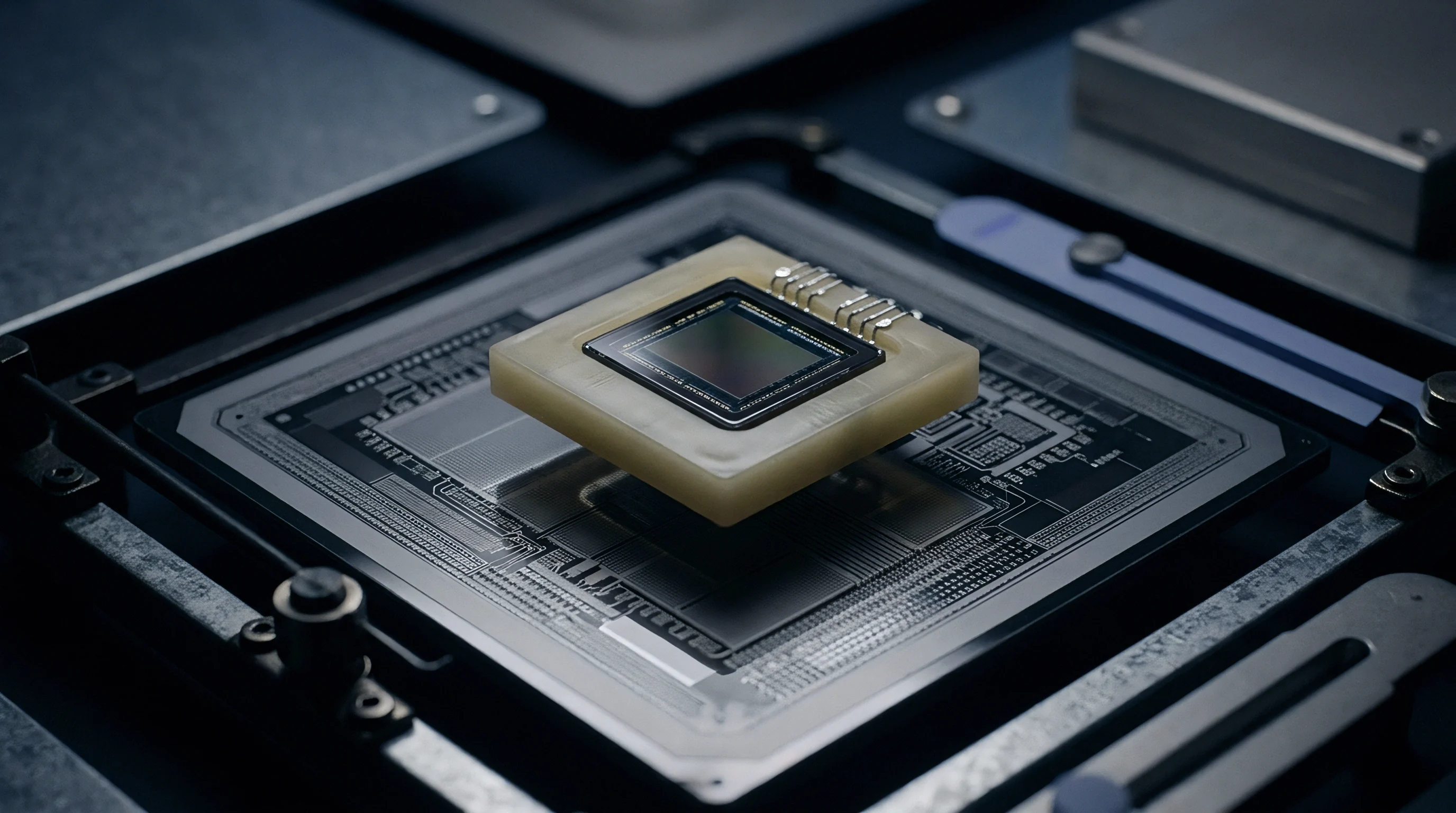
Direct real-time characterization of viscoelastic relaxation over five to ten years of operational life is unfeasible during standard development schedules. Instead, material metrologists apply the Time-Temperature Superposition Principle to accelerate testing. This principle relies on the equivalence between operational temperature shifts and timescale changes in thermorheologically simple polymers: elevated temperatures enhance molecular segment mobility, compressing relaxation timescales without altering underlying deformation mechanisms.
Dynamic mechanical analysis measures storage modulus G’ and loss modulus G” over a practical laboratory frequency range, typically from 0.1 hertz to 100 hertz, across a series of isothermal temperature steps. Translating isothermal frequency curves horizontally along the logarithmic time or frequency axis aligns overlapping segments into a single master curve at a designated reference temperature T_ref.
The horizontal translation distance applied to each isothermal curve equals the dimensionless logarithmic shift factor log10(a_T). Above the glass transition temperature T_g, shift factors follow the empirical Williams-Landel-Ferry equation:
log10(a_T) = -C1 (T – T_ref) / (C2 + T – T_ref)
The empirical parameters C1 and C2 represent material-specific constants calibrated at reference temperature T_ref. Below the glass transition temperature, where glassy polymer kinetics dominate, shift factor progression transitions to an Arrhenius formulation:
ln(a_T) = (E_a / R) (1 / T – 1 / T_ref)
The parameter E_a represents the apparent activation energy for sub-glass transition molecular segment relaxation, R represents the universal gas constant, and T represents absolute temperature in kelvin.
Epoxy molding compounds exhibiting a twenty degree glass transition shift under moisture saturation alter Prony relaxation times by two orders of magnitude at eighty five degrees Celsius.
Isothermal DMA Characterization Protocols
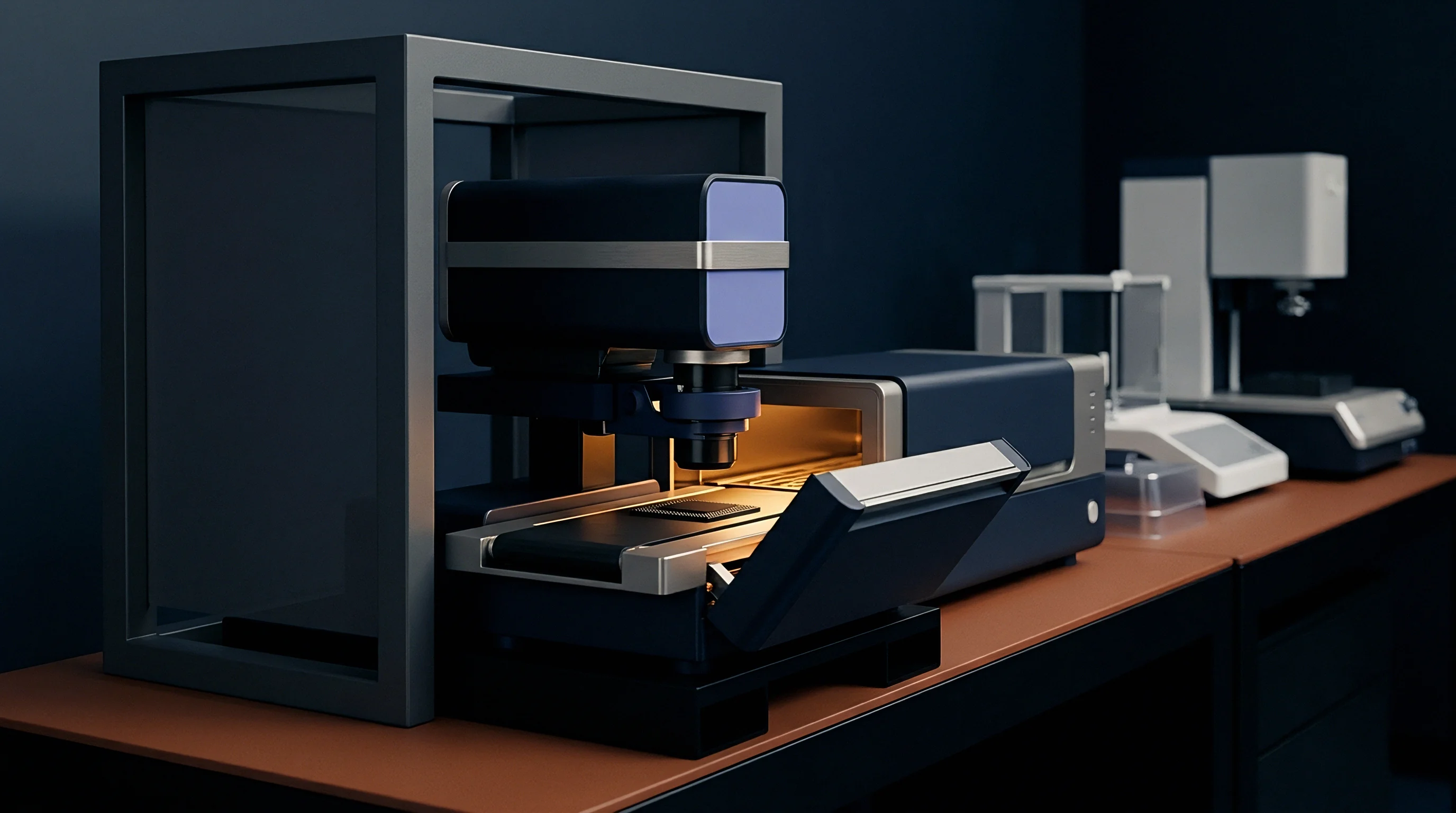
Constructing reliable master curves and extracting accurate Prony parameters demands precise experimental measurement protocols on calibrated dynamic mechanical analyzers.
- Machining rectangular beam specimens from fully cured polymer stock to uniform dimensions within a 0.02 millimeter tolerance boundary.
- Loading the specimen into a dual cantilever or three-point bending test fixture within the temperature-controlled chamber of an accredited dynamic mechanical analyzer.
- Equilibrating the sample at the lowest target temperature, typically minus 50 degrees Celsius, for a minimum soak window of 15 minutes.
- Applying an oscillatory strain sweep from 0.01 percent to 0.1 percent strain amplitude to verify linear viscoelastic response limits.
- Executing a multi-frequency dynamic test sweep from 0.1 hertz to 50 hertz across stepped temperature increments of 5 degrees Celsius up to 180 degrees Celsius.
- Extracting storage modulus G’ and loss modulus G” frequency curves for each isothermal step using calibrated instrument software.
- Shifting isothermal data segments manually or via non-linear least-squares fitting algorithms relative to chosen reference temperature T_ref to construct a continuous master curve.
- Performing discrete mathematical optimization to fit the normalized Prony series parameters to the resulting master relaxation curve.
Water molecules penetrating epoxy packaging networks act as plasticizers, depressing the glass transition temperature and shifting viscoelastic relaxation rates toward shorter timescales. Standard dry dynamic mechanical analysis curves register packaging compliance while overlooking the moisture plasticization that accelerates operational drift under humid ambient service conditions.
| Epoxy Formulation | Glass Transition Tg (deg C) | Reference Temp T_ref (deg C) | WLF Constant C1 | WLF Constant C2 (K) | Activation Energy Ea (kJ/mol) |
|---|---|---|---|---|---|
| High-Purity Die Attach Epoxy | 145 | 145 | 14.2 | 52.4 | 168 |
| Low-Stress Mold Compound | 160 | 160 | 16.8 | 48.1 | 185 |
| Underfill Resins Type A | 120 | 120 | 12.5 | 45.0 | 142 |
| Encapsulation Epoxy Type B | 95 | 95 | 11.1 | 38.6 | 125 |

Solver
Numerical Integration of Hereditary Integrals
Finite element implementation of Prony series viscoelasticity converts historical stress-strain convolution integrals into incremental state-variable recursive algorithms. Direct numerical integration of hereditary integrals across extended loading histories would require storing the entire strain history for every integration point in a mesh, consuming excessive computer memory and execution time. Commercial solvers avoid this memory overhead by utilizing a strain-increment formulation.
The solver updates internal viscoelastic state variables at the end of each incremental time step delta_t based solely on strain increments accumulated during that specific time interval and the state variable values from the preceding step. For a single Maxwell branch, the recursive state variable update takes the functional form:
S_i(t + delta_t) = exp(-delta_t / tau_i) S_i(t) + g_i G_0 delta_epsilon
The variable S_i represents the internal stress state vector carried by the i-th Maxwell element, while delta_epsilon represents the mechanical strain increment tensor calculated across time step delta_t. Summing internal stress states S_i across all N terms and adding the instantaneous elastic stress contribution yields the updated total stress vector at time t plus delta_t. Mesh convergence studies must evaluate element formulation sensitivity near rigid die boundaries to prevent artificial stress concentration artifacts.
- Volumetric Thermal Expansion accounts for isotropic dimensional change driven by temperature swings combined with linear coefficient of thermal expansion values.
- Chemical Cure Shrinkage incorporates volumetric strain reduction occurring during polymer network cross-linking prior to thermal cooling.
- Viscoelastic Strain Accumulation tracks time-dependent creep strain vectors calculated recursively by the Prony solver core.
- Geometrical Non-Linearity accounts for large structural deflections and warping shifts occurring across thin substrate packages.
Standard IEC 60749 twenty six compliance testing without long term stress modeling misses zero point wander caused by sub glass transition polymer relaxation.

Piezoresistive Strain Mapping in Finite Element Analysis
Calculating packaging stress decay allows direct mapping of time-dependent stress tensors onto sensor active regions. Silicon piezoresistive pressure sensors rely on p-type piezoresistors diffused into an n-type diaphragm surface along specific crystallographic orientations, typically the direction on a (100) silicon plane. Longitudinal and transverse stress components applied to the piezoresistor modify its electrical resistivity through the piezoresistive coefficient matrix.
Change in electrical resistance delta_R relative to un-stressed resistance R_0 for a Wheatstone bridge resistor arm follows the piezoresistive coupling equation:
delta_R / R_0 = pi_l sigma_l + pi_t sigma_t + pi_z sigma_z
The parameters pi_l, pi_t, and pi_z represent the piezoresistive coefficients along longitudinal, transverse, and normal directions relative to current flow, while sigma_l, sigma_t, and sigma_z represent the corresponding normal stress components acting on the piezoresistors. When die-attach packaging stresses relax viscoelastically, sigma_l and sigma_t decay over time. As a result, delta_R / R_0 drifts, driving offset voltage drift across the Wheatstone bridge output even when applied pressure remains perfectly constant.
Assume a MEMS pressure sensor die attached with silver-filled epoxy exhibiting an initial compressive die surface stress of minus 45 megapascals post-cure cooling. Over 2,000 operating hours at 85 degrees Celsius, viscoelastic stress relaxation reduces compressive surface stress to minus 32 megapascals, representing a 13 megapascal stress drop. With a typical longitudinal piezoresistive coefficient pi_l of 71.8 x 10^-11 per pascal, this packaging stress decay causes an uncompensated resistance shift delta_R / R_0 of approximately 0.93 percent.
In a full-bridge sensor configuration with 100 millivolt full-scale output under 100 kilopascal applied pressure, this package-induced relaxation manifests as a zero offset drift of 1.86 millivolts, representing a 1.86 percent full-scale measurement error solely attributable to packaging adhesive relaxation.
A rigorous finite element analysis workflow inputs discrete Prony parameters, evaluates recursive stress decay step-by-step, maps stress tensor transformations to piezoresistive bridge locations, and predicts long-term offset wander across the full specified operating thermal envelope.


Offset

Package Relaxation Effects on Output Zero Stability
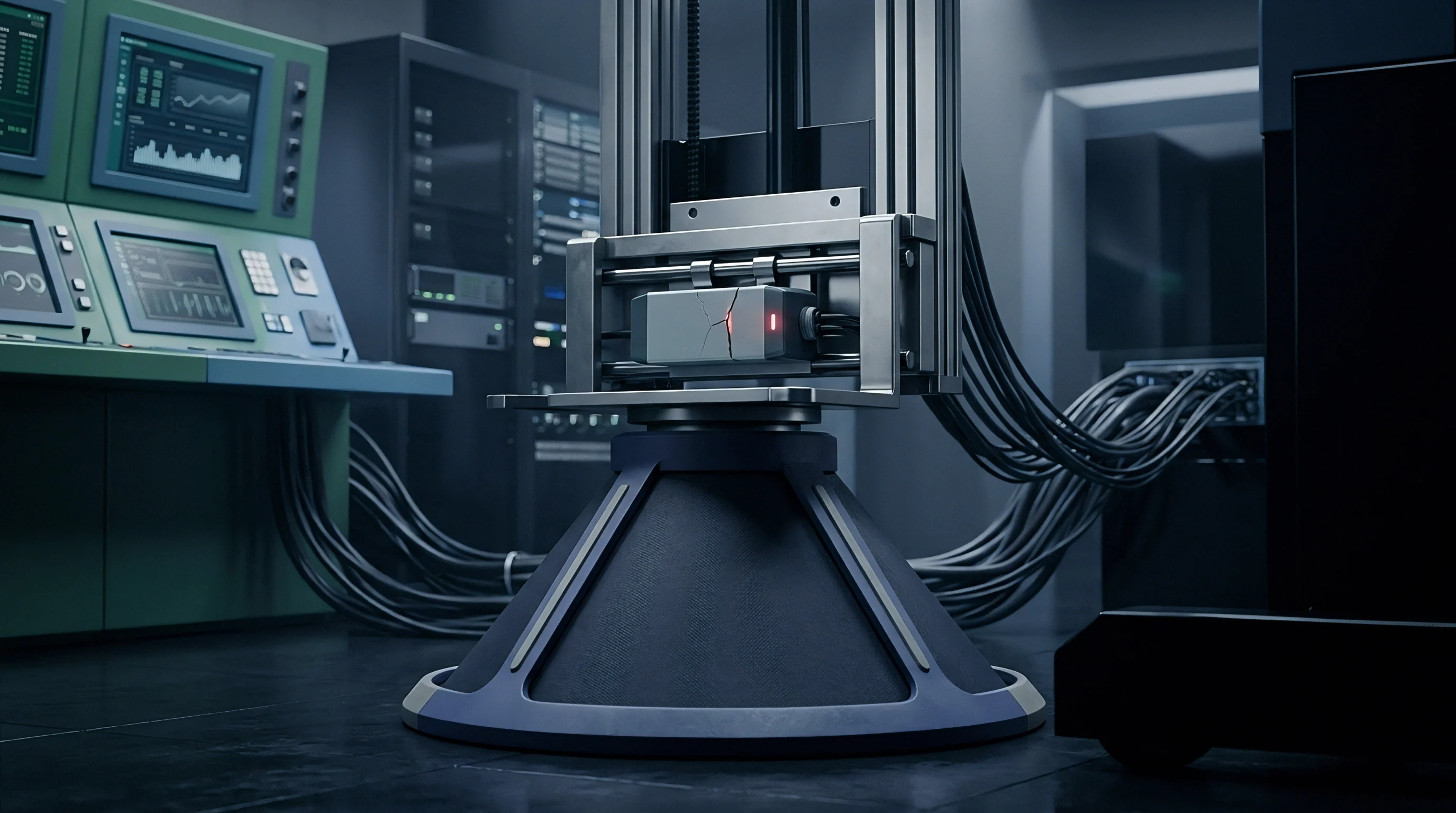
Transducer performance datasheets state static accuracy figures valid at the moment of factory calibration. Field service exposes packaging materials to continuous thermomechanical stresses, driving long-term baseline wander. Packaging stress relaxation manifests primarily as zero-point offset drift, span sensitivity drift, and thermal hysteresis loop expansion.
Zero-point offset drift represents the changing electrical output of an unpressurized transducer over time. When packaging stress relaxes, the static mechanical background load on the active sensor element shifts, producing a false pressure signal. Span sensitivity drift occurs when packaging stress alters the flexural rigidity of thin sensor diaphragms or changes piezoresistive coupling coefficients through non-linear piezojunction effects.
Piezoresistive silicon diaphragms measure mechanical packaging stresses with the same sensitivity as applied fluid pressure.
Accelerated Aging and Thermal Conditioning Strategies
Mitigating package-induced zero drift in high-precision transducers requires structured thermal conditioning protocols prior to factory calibration. Thermal bake stabilization accelerates early high-rate viscoelastic relaxation, forcing packaging epoxies past the initial steep region of their modulus decay curve.
- High Temperature Storage Stabilization bakes assembled transducer core sub-assemblies at elevated temperatures to dissipate initial cure residual stresses prior to calibration.
- Thermal Cycling Pre-Conditioning subjects packages to repeated temperature extremes to break weak interfacial bonds and stabilize polymer network relaxation rates.
- Zero-Point Burn In Monitoring tracks baseline voltage drift continuously during thermal stabilization to identify non-conforming units exhibiting abnormal creep rates.
- Post Calibration Drift Characterization measures residual baseline creep across post-bake storage intervals to establish traceable stability uncertainties.
Holding packaging materials at elevated temperatures for 100 to 200 hours dissipates high early stress relaxation rates, driving the material into its flat equilibrium relaxation regime where subsequent operational drift rates drop by up to an order of magnitude.
| Sensor Transducer Type | Packaging Encapsulation Type | Initial Packaging Stress (MPa) | 1000-Hour Stress Decay (%) | Uncompensated Zero Drift (% FS) | Post-Bake Zero Drift (% FS) |
|---|---|---|---|---|---|
| Piezoresistive Pressure Sensor | Silver-Filled Epoxy Die Attach | -42.5 | 28.2 | 1.65 | 0.18 |
| Capacitive Force Transducer | Rigid Underfill Matrix | -28.0 | 18.5 | 0.82 | 0.09 |
| MEMS Strain Gauge Bridge | Epoxy Glob-Top Encapsulant | -65.0 | 36.4 | 2.40 | 0.31 |
| Optical MEMS Pressure Element | Soft Silicone Gel Potting | -2.1 | 8.0 | 0.12 | 0.03 |
How do environmental humidity excursions interact with thermal stabilization cycles to modify long-term zero drift limits in non-hermetic sensor packages?

Dossier

Material Data Sheet Requirements for Viscoelastic Parameters
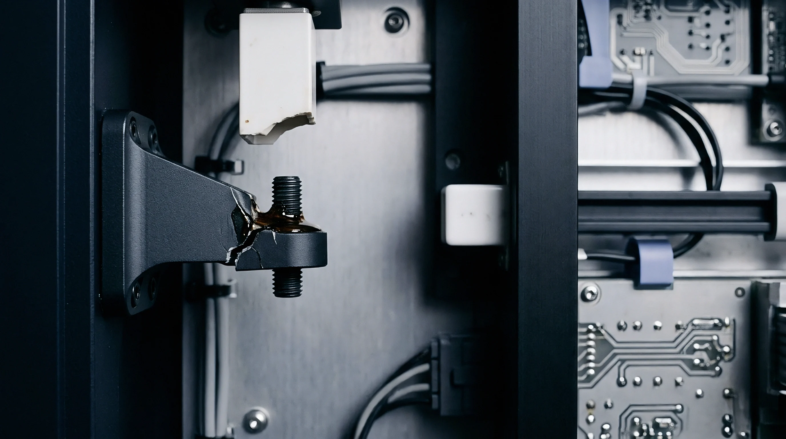
Procurement specifications for high-precision sensor packaging polymers must mandate complete viscoelastic characterization dossiers rather than static single-point mechanical properties. Conventional material datasheets quote static room-temperature tensile modulus, glass transition temperature by differential scanning calorimetry, and linear coefficient of thermal expansion. These static figures provide zero insight into time-dependent stress decay rates or long-term operational sensor stability.
Technical buyers specify full dynamic mechanical analysis characterization reports certified by ISO/IEC 17025 accredited testing laboratories. Sourcing agreements require raw polymer suppliers to deliver tabular storage and loss moduli frequency sweeps, calibrated WLF shift constants, and calculated Prony series coefficients spanning target operational temperature limits.

Quality Verification Procedures for Incoming Encapsulants
Quality assurance teams verify incoming resin lots to ensure consistency in viscoelastic relaxation parameters across manufacturing runs. Subtle variations in resin cross-linking density, filler loading fractions, or catalyst ratios alter glass transition behavior and change relaxation time scales.
Incoming lot verification testing utilizes standardized differential scanning calorimetry and dynamic mechanical analysis protocols. Acceptance criteria establish explicit tolerance bands around reference Prony series parameters, ensuring that batch-to-batch polymer variations do not drive uncompensated baseline drift in calibrated sensor assemblies.
Because recalibration intervals double operational costs, sourcing specifications incorporate strict material verification clauses governing organic packaging compounds.
Under Clause 8.3 of quality procurement specifications for precision sensor packaging polymers, suppliers shall provide calibrated N-term Prony series shear modulus parameters (g_i, tau_i) and Williams-Landel-Ferry constants (C1, C2) derived from ISO/IEC 17025 accredited dynamic mechanical analysis test reports across the specified operating temperature range, and any unannounced alteration to polymer formulation, filler content, or cure kinetics that alters calculated 1000-hour stress relaxation values by more than 5 percent shall constitute a non-conformance invalidating lot acceptance.