Calibrating Precision Resistance Standards across Ambient Thermal Ranges
Ambient thermal calibration demands fitting parabolic alloy coefficients and correcting thermoelectric offsets to bound resistance drift under operational swings.


Alloy

Metallurgical Phase Stability
Solid-solution resistance materials achieve low temperature sensitivity through precise composition control and thermal annealing. Precision wire-wound standards rely heavily on quaternary nickel-chromium alloys containing copper and aluminum, commercially designated as Evanohm or NiCr40AlCu. Sheet foil standards predominantly employ nickel-chromium or copper-manganese-nickel formulations such as Manganin and Zeranin.
Crystalline lattice strain induced during cold drawing or rolling, followed by stress-relief heat treatment above 350°C, dictates the electrical behavior of these metals. Unannealed wire retains high internal dislocation density, causing unpredictable zero-point resistance wander during ambient shifts.
Chemical composition dictates the second-order thermal characteristics of these alloys. Manganese content in Manganin shifts the parabolic peak of resistance toward room temperature, while grain boundary stabilization prevents localized oxidation. In Evanohm, heat treatment induces short-range atomic ordering to adjust the temperature coefficient of resistance across standard laboratory thermal ranges.
Uncontrolled ambient excursions alter this ordered state over time, generating micro-ohmic baseline drift that invalidates room-temperature calibration adjustments.
Parabolic Temperature Coefficients
Thermal sensitivity in high-precision resistors is non-linear across operational ambient ranges. Metrological conventions model resistance variation as a second-order polynomial centered at a standard reference baseline, typically 23°C or 25°C. The standard formulation defines resistance at temperature T according to the reference temperature T0 and the primary temperature coefficients:
R(T) = R(T0)
Alpha represents the first-order temperature coefficient expressed in parts per million per kelvin (ppm/K), while beta denotes the second-order coefficient in parts per million per kelvin squared (ppm/K^2). In high-grade Evanohm standards, alpha is trimmed near zero at 23°C, ranging between -0.5 ppm/K and +0.5 ppm/K. Beta remains consistently negative, typically falling between -0.005 ppm/K^2 and -0.03 ppm/K^2. Manganin exhibits a larger negative beta, near -0.03 to -0.05 ppm/K^2, causing its resistance curve to drop rapidly as ambient temperature deviates from its peak value.
The zero-TCR crossover temperature of Evanohm shifts by up to 1.5°C following prolonged exposure to temperatures above 40°C.
Laboratory ambient swings between 18°C and 28°C impose quantifiable shifts on uncorrected standard values. Evaluating a 10 kilohm standard with an alpha of +0.2 ppm/K and a beta of -0.015 ppm/K^2 at an ambient temperature of 28°C yields a baseline deviation relative to 23°C. A temperature differential of +5°C produces a first-order change of +1.0 ppm and a second-order term of -0.375 ppm, giving a combined departure of +0.625 ppm (6.25 milliohms). Leaving either parameter uncorrected creates systemic errors across varying laboratory environments.
Thermal Equilibrium and Strain Mechanisms
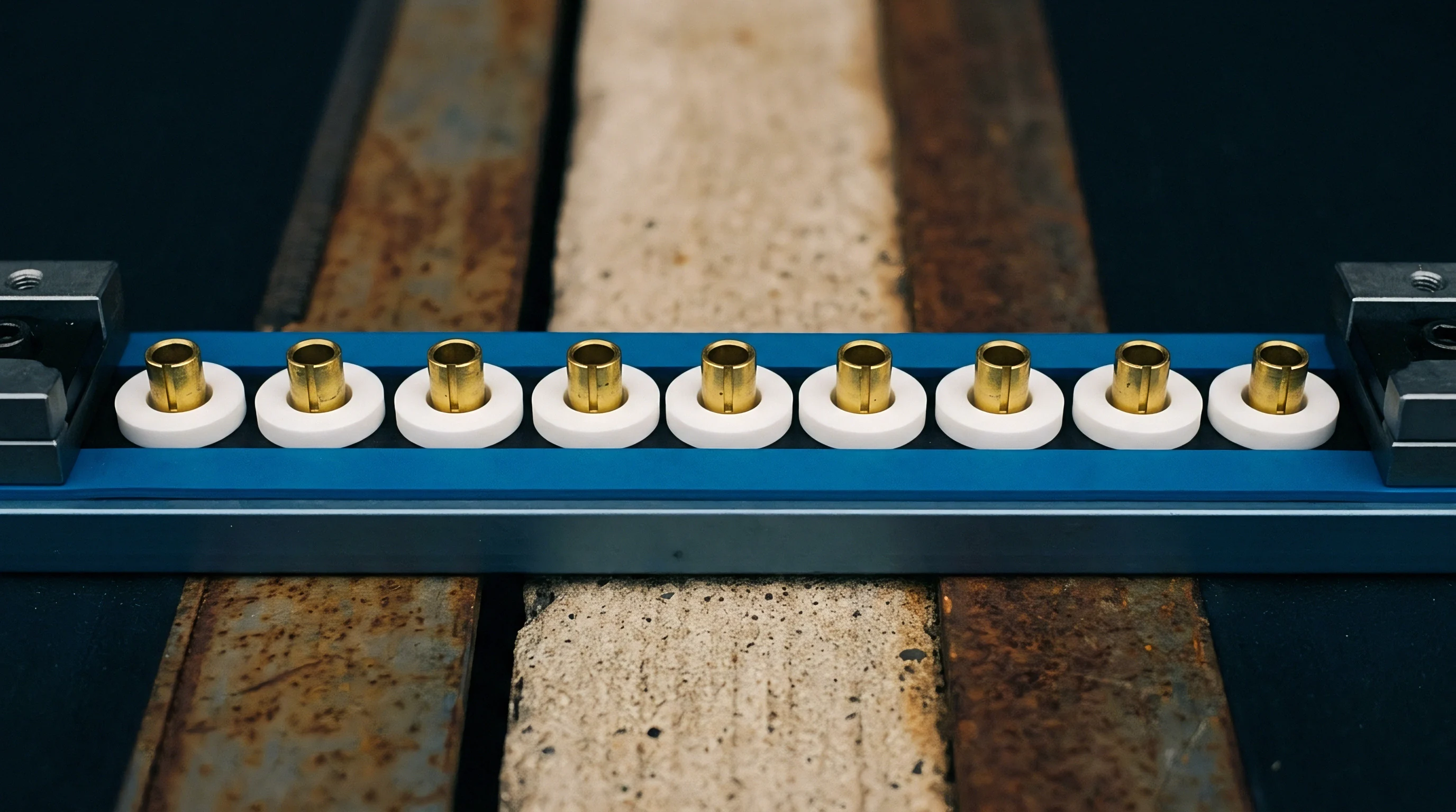
Mechanical stress alters the electrical resistivity of precision alloys through piezoresistive coupling. Standard resistors enclose element assemblies within oil-filled or hermetically sealed stainless steel housings to damp environmental changes. Copper lead wires pass through ceramic glass seals, matching the thermal expansion coefficient of the containment shell to minimize physical strain on the primary element.
Differential expansion between the alloy element, internal support mandrels, and insulating wraps introduces localized stress during rapid room thermal cycling.
Time constants for thermal stabilization vary substantially across physical constructions. Bare wire coils suspended in oil achieve equilibrium rapidly due to high fluid heat transport, reaching stability within twenty minutes of ambient shifts. Enclosed air-insulated foil standards require four to six hours to equalize internal thermal gradients following a 5°C ambient shift.
Calibration protocols executed before achieving full structural equilibrium register transient stress states rather than true material baseline resistance.
Single-point factory measurements can suggest zero temperature sensitivity across wide operating bands, but these readings reflect isolated zero-crossing points on a parabolic curve rather than uniform insensitivity across thermal ranges.

Wire

Winding Geometries and Thermal Dissipation
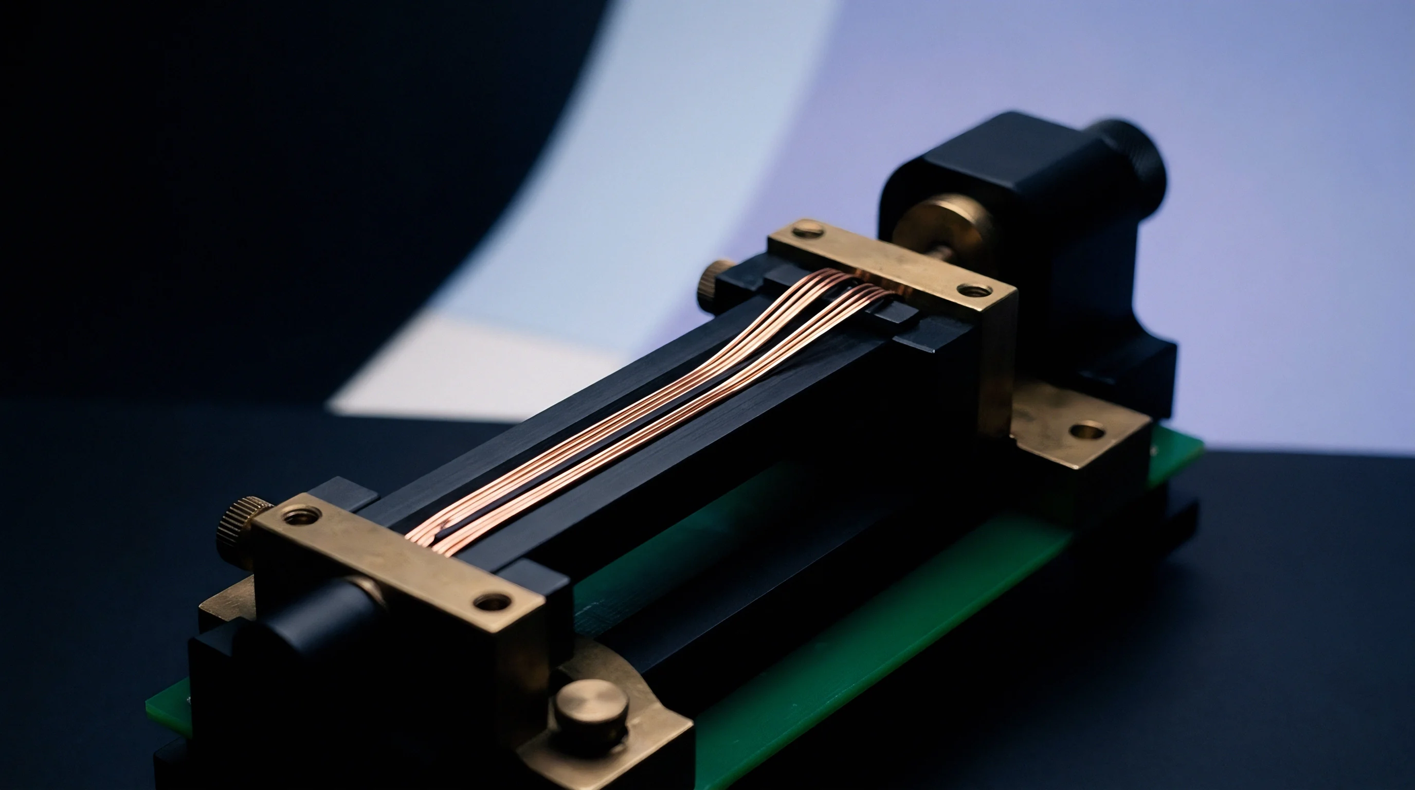
Mechanical winding geometry determines both inductive reactivity and heat removal efficiency in wire-wound standards. Bifilar and Ayrton-Perry winding methods cancel parasitic self-inductance by placing adjacent wire turns with opposing current paths in close spatial contact. This close proximity increases thermal coupling between adjacent conductors, concentrating dissipated power within internal layers.
Heat generated by test currents escapes outward through insulating enamel, support mandrels, and fluid media.
Self-heating raises the internal wire temperature above the surrounding ambient medium. The power coefficient of resistance quantifies this internal thermal rise relative to applied electrical power. The relationship converts applied excitation current into equivalent ambient shift:
Delta T = P R_th
R_th represents the thermal resistance of the assembly in kelvins per watt, while P denotes applied power in watts. A 100-ohm standard carrying 10 milliamperes dissipates 10 milliwatts. With an internal thermal resistance of 15 K/W, the wire core operates 0.15°C above the external environment.
If the element possesses a temperature coefficient of -2 ppm/K, self-heating introduces a baseline offset of -0.3 ppm regardless of external climate stability.
| Enclosure Architecture | Internal Medium | Thermal Time Constant (t63) | Core Thermal Resistance | Maximum Recommended Power |
|---|---|---|---|---|
| Thomas-Type Sealed Cylinder | Mineral Oil | 18 minutes | 8.5 K/W | 100 mW |
| Hermetic Air Standard | Dry Nitrogen | 210 minutes | 42.0 K/W | 10 mW |
| Open-Frame Card Standard | Ambient Air | 45 minutes | 28.0 K/W | 25 mW |
| Direct Immersed Foil Standard | Silicone Fluid Bath | 4 minutes | 2.1 K/W | 500 mW |

Parasitic Thermal Voltage Generation
Dissimilar metal junctions inside the resistor assembly generate parasitic thermoelectric voltages through the Seebeck effect. Connecting Evanohm resistance wire directly to internal copper posts creates thermocouple pairs producing approximately 1 to 3 microvolts per kelvin temperature difference across the junction. Thermal gradients across the housing cause unequal heating between opposing junction nodes, establishing persistent internal DC offsets.
Direct current measuring systems interpret Seebeck voltages as resistance shifts unless cancelled by measuring protocols. A 2-microvolt thermal EMF across a 10-ohm standard measured with a 1-milliampere test current generates a 2-milliohm measurement error, representing a 200 ppm calibration distortion. Reversing current direction isolates true resistive voltage drops from persistent thermal EMFs.
Asymmetrical ambient heating undermines this cancellation if thermal gradients change faster than the measurement system polarity switching cycle.
Environmental Degradation Modes
Precision wire assemblies degrade through environmental and mechanical mechanisms during ambient thermal cycling:
- Intergranular Oxidation selectively attacks alloy constituents along microscopic grain boundaries, increasing baseline resistance over operational service life.
- Insulation Resistance Breakdown occurs when moisture penetrates porous varnish layers, creating parallel high-resistance leakage paths across adjacent turns.
- Mandrel Stress Coupling transfers mechanical expansion forces from internal support spools into the resistance wire, shifting the zero-strain thermal reference point.
- Sublimation of Volatile Binders deposits insulating residues on internal contact surfaces, altering low-current contact resistance in terminal junctions.
Avoiding tight bending radii during manufacturing prevents localized strain concentrations that accelerate these physical degradation modes.

Frost
Sub-Ambient and Extended Thermal Operation
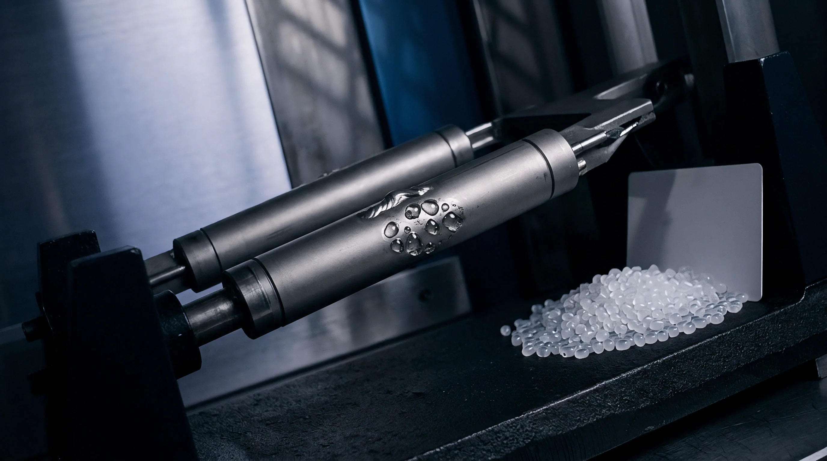
Operating precision resistance standards below dew point temperatures introduces severe insulation degradation risks. Moisture condensation on housing terminals creates low-resistance parallel paths, degrading isolation resistance between primary terminals and ground. Pure water condensation forms a surface leakage layer with surface resistivity dropping from tens of teraohms per square to megaohms per square, reducing effective measured resistance by hundreds of parts per million.
Frost accumulation on non-hermetic terminals induces severe physical pressure on exposed wire leads during freeze-thaw cycles. Micro-cracks develop in protective conformal coatings, allowing moisture ingress into the internal resistance element matrix. Moisture absorption in organic insulating materials causes swelling, generating mechanical strain on fine resistance wire coils.
Sub-ambient calibration requires sealed environmental test chambers purged with dry nitrogen maintaining a dew point below -40°C.
ISO/IEC 17025 accreditation scopes mandate explicit ambient relative humidity bounds between 30% and 55% during standard resistor transfer calibrations.
Thermal Hysteresis and Excursion Memory
Thermal cycling beyond tightly controlled laboratory bounds causes permanent or semi-permanent baseline resistance offsets. Thermal hysteresis describes the failure of a standard resistor to return to its original resistance value at 23°C after exposure to elevated or sub-ambient temperatures. Physical mechanisms include dislocation movement in the metal lattice, grain boundary relaxation, and relief of structural mounting stresses.
Measuring thermal hysteresis involves logging baseline resistance at 23°C, heating the standard to 50°C for twenty-four hours, cooling back to 23°C, and tracking recovery over time. Evanohm wire standards display a short-term hysteresis loop ranging from 0.05 ppm to 0.4 ppm following a 25°C thermal excursion. The recovery phase often extends over days or weeks as internal mechanical stress relaxes toward equilibrium.
Ignoring thermal recovery time frames leads to false drift readings following transit between field sites and temperature-controlled laboratories.

Bridge
Direct Current Comparator Bridges
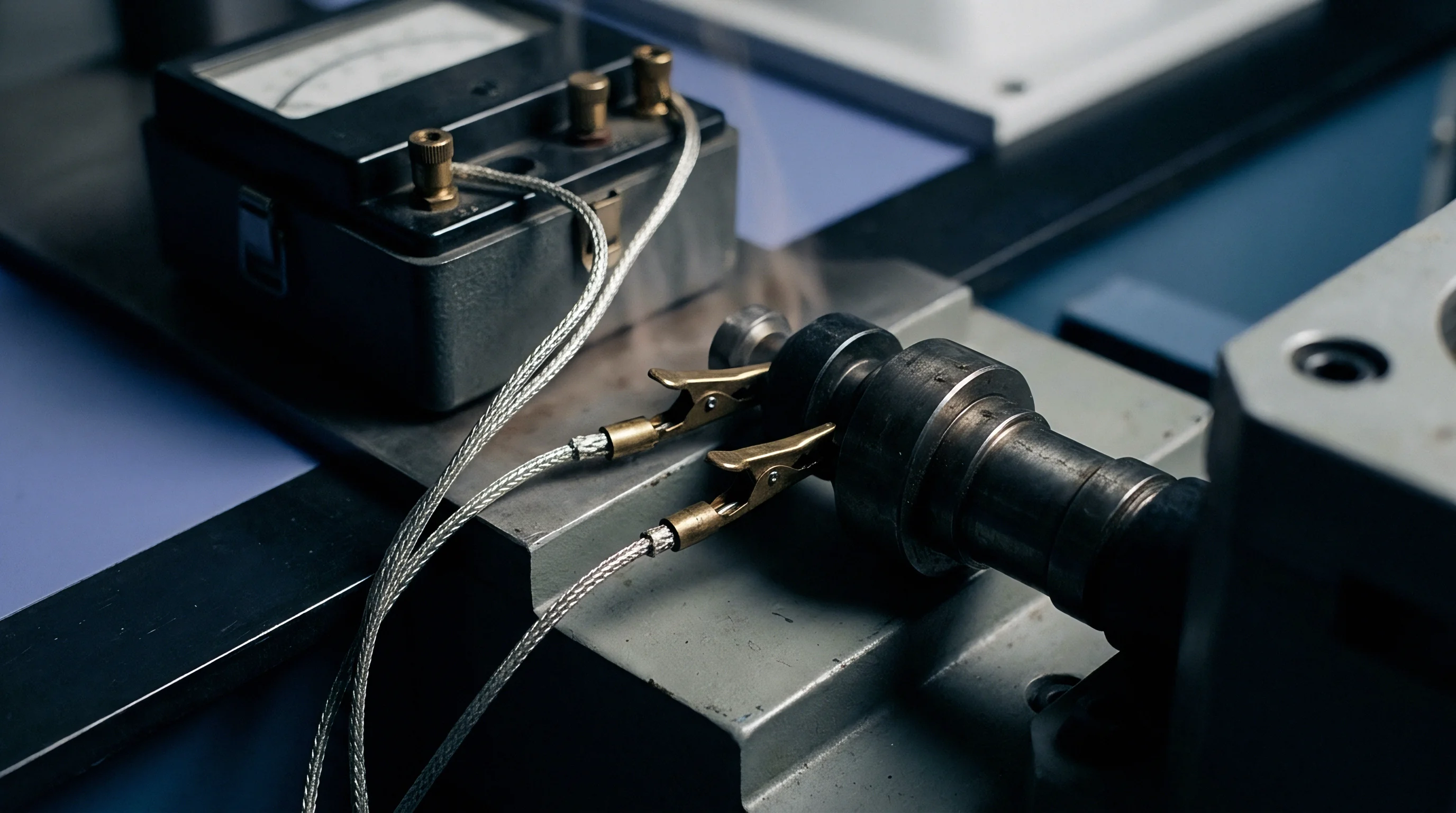
Direct Current Comparator (DCC) bridges represent the primary metrological method for calibrating resistance standards across variable thermal environments. DCC technology relies on balance of magnetic fluxes generated by direct currents passing through precision-ratio turns windings on a high-permeability toroidal core. Ratio accuracy depends on physical turn ratios rather than unstable passive resistance components, rendering the bridge ratio virtually immune to ambient laboratory thermal changes.
The primary current I1 flows through standard Rx, while secondary current I2 passes through standard Rs. An automated feedback loop adjusts I2 to maintain zero net magnetic flux in the toroidal core. The fundamental measurement relationship follows the turns ratio:
Rx / Rs = N2 / N1
Modern automated DCC bridges achieve ratio uncertainties below 0.01 ppm at room temperature. Measuring standards inside climate-controlled chambers while maintaining the DCC bridge electronics at ambient lab temperature decouples bridge circuit thermal drift from standard element thermal performance.
Reversal Protocols and Thermal EMF Elimination
Precise thermal characterization demands active elimination of static and drifting thermoelectric voltages. Automated current reversal sequences switch primary measurement current polarity at fixed intervals, typically every eight to sixty seconds. The bridge averages forward and reverse voltage drop measurements to isolate pure resistive impedance:
V_meas_forward = I R + V_emf
V_meas_reverse = -I R + V_emf
V_true = (V_meas_forward – V_meas_reverse) / 2 = I R
Linear drift in thermoelectric potential requires higher-order mathematical filtering. Polynomial extrapolation models track background thermal EMF evolution during current switching cycles. Fast-switching solid-state current commutators minimize measurement dead time, preventing thermal recovery transients from corrupting averaged data points.
Lead Resistance and Guarded Terminal Networks
Four-terminal (Kelvin) connection configurations eliminate lead wire resistance errors during wide ambient testing. Separate current-carrying and voltage-sensing leads isolate lead wire resistance from measured standard values. Variable ambient temperatures alter test lead wire resistance by up to 0.4% per kelvin for standard copper cable, introducing significant measurement errors in two-terminal measurement setups.
| Error Source | Physical Origin | Typical Magnitude (Uncompensated) | Mitigation Technique | Residual Uncertainty |
|---|---|---|---|---|
| Parasitic Thermal EMF | Seebeck potential across copper-alloy junctions | 0.5 uV to 5.0 uV | Square-wave current reversal | < 0.002 ppm |
| Current Lead Resistance | Ohmic voltage drop in test cables | 10 mOhm to 500 mOhm | Four-terminal Kelvin connection | < 0.001 ppm |
| Insulation Leakage | Parallel humidity film across terminals | 10 Gohm to 1 Tohm path | Active terminal guard driving | < 0.005 ppm |
| Self-Heating Drift | Joule heating in fine wire element | 0.1 ppm to 2.0 ppm | Dual-current power extrapolation | < 0.010 ppm |
Elevated humidity during thermal cycles directly degrades automated bridge measurements.
High humidity creates parasitic leakage paths between signal leads and earth ground. Active guard driving places a low-impedance shield around inner signal conductors, holding the shield at identical electrical potential to eliminate current flow through insulation paths.
Unchecked insulation degradation eventually exceeds the drive capability of active guard amplifiers, causing subtle bridge balance errors.

Arithmetic
Uncertainty Budget Structure
Evaluating standard resistance uncertainty across ambient thermal ranges requires compiling a formal uncertainty budget compliant with the ISO/IEC Guide to the Expression of Uncertainty in Measurement (GUM). Individual uncertainty contributions enter the budget as standard uncertainties u(xi) categorized as Type A (evaluated by statistical analysis of series of observations) or Type B (evaluated using external calibration data, physical constants, or manufacturer specifications).
Combined standard uncertainty u_c(R) aggregates individual components through square-root sum-of-squares addition, assuming independent, uncorrelated variables:
u_c(R) = sqrt( sum )
Sensitivity coefficients c_i convert component dimensions into resistance variance equivalents (ppm or milliohms). The expanded uncertainty U uses a coverage factor k=2, defining an interval with an approximate 95% level of confidence.
Worked Calibration Calculation
Consider calibrating a 1000-ohm precision standard resistor across an ambient climate range of 18°C to 28°C inside an environmental test chamber. The reference standard resistor possesses a certified value of 1000.00012 ohms with an expanded calibration uncertainty of 0.20 ppm (k=2) at 23.0°C. Primary parameters and uncertainties include:
- Reference Standard Value carries a standard uncertainty u(R_std) equal to 0.20 / 2 = 0.10 ppm.
- Reference Drift between annual calibration cycles contributes an estimated standard uncertainty u(R_drift) of 0.08 ppm based on historical calibration records.
- Bridge Ratio Accuracy operating in direct comparator mode contributes a Type B standard uncertainty u(Ratio) of 0.03 ppm.
- Thermal Chamber Gradient introduces a temperature uncertainty of +/-0.15°C at the sensor location, with standard uncertainty u(T_bath) = 0.15 / sqrt(3) = 0.0866°C assuming a rectangular distribution.
- Temperature Coefficient Sensitivity for an element with alpha = +0.8 ppm/K and u(alpha) = 0.05 ppm/K translates temperature uncertainty into resistance uncertainty: c_T = alpha = 0.8 ppm/K; u(R_temp) = 0.8 0.0866 = 0.0693 ppm.
- Self-Heating Uncertainty under 1-milliwatt test power contributes u(R_power) equal to 0.02 ppm.
- Type A Measurement Repeatability over ten automated reversal cycles yields a standard deviation of the mean u(R_typeA) equal to 0.015 ppm.
Summing these squared standard uncertainties yields the combined standard uncertainty:
u_c^2 = (0.10)^2 + (0.08)^2 + (0.03)^2 + (0.0693)^2 + (0.02)^2 + (0.015)^2
u_c^2 = 0.0100 + 0.0064 + 0.0009 + 0.004802 + 0.0004 + 0.000225 = 0.022727 ppm^2
u_c = sqrt(0.022727) = 0.1508 ppm
Multiplying by coverage factor k=2 establishes the expanded uncertainty U = 0.3016 ppm. For a 1000-ohm nominal value, the calibration certificate states 1000.00012 ohms +/- 0.00030 ohms (or +/- 0.30 ppm) at 23.0°C under specified thermal conditions.
ISO/IEC 17025 standard clause 7.8.4.1 mandates reporting both the expanded uncertainty and the specific coverage factor applied to every reported resistance standard calibration figure.

Yield

Guardbanding and Commercial Compliance
Uncertainty in ambient thermal calibration directly impacts commercial product compliance decisions. Guardbanding shrinks acceptable test tolerance limits below manufacturer datasheet specifications to account for measurement uncertainty. A high standard measurement uncertainty reduces manufacturing yield by causing acceptable precision resistors to fail incoming quality verification.
ILAC-G8 guidelines establish formal decision rules for pass/fail assessments. Binary acceptance with a simple acceptance limit requires the measured resistance value plus expanded measurement uncertainty to fall entirely within specified product tolerance bounds:
Lower Tolerance Limit + U <= Measured Value <= Upper Tolerance Limit – U
When measuring a 0.001% (10 ppm) tolerance resistor, an expanded measurement uncertainty of 3 ppm consumes 30% of the entire allowable tolerance band on each side. The usable production band narrows to 4 ppm total width centered at nominal value. Tightening ambient laboratory thermal control reduces measurement uncertainty U, expanding usable acceptance limits and increasing production yield.
Cost Trade-Offs in Thermal Infrastructure
Maintaining primary metrology standards requires evaluating physical infrastructure investment against calibration uncertainty penalties. Fluid-bath temperature control achieves exceptional stability, holding fluid temperatures within +/- 0.002°C using active proportional-integral-derivative thermal management. Oil bath systems carry high acquisition costs, continuous maintenance burdens, and fluid handling hazards.
Modern hermetic foil standards operating inside temperature-controlled air enclosures provide alternative options with lower ongoing support costs.
Air chambers holding baseline temperature within +/- 0.05°C incur one-fourth the capital cost of high-precision oil bath setups. Air systems introduce larger thermal gradients and longer thermal equilibrium time frames. Field calibration laboratories balance these operational realities against target test uncertainty ratios.
Selecting air-insulated standards with small temperature coefficients yields acceptable test uncertainty ratios for 100 ppm commercial workloads without oil bath investments.
Recalibration interval management dictates long-term cost of ownership for precision standards. Standards cycled through non-controlled field ambient ranges demonstrate accelerated baseline drift rates, requiring shortened six-month calibration cycles to maintain certificate validity. Standards permanently maintained inside tight laboratory thermal bounds maintain predictable linear drift rates, justifying extension to twenty-four-month recalibration intervals under accredited quality management programs.