Static Gravity Vector Calibration for Triaxial MEMS Accelerometers
Static 12-parameter gravity vector calibration isolates MEMS accelerometer zero offset, scale factor, and axis misalignment to reach sub-millig precision.


Frame
MEMS accelerometers measure displacement through changes in differential capacitance across micro-machined silicon comb structures. External forces move the suspended proof mass, altering the spacing between interdigitated mechanical fingers. Signal conditioning circuitry converts these capacitance variations into analog voltages before high-resolution analog-to-digital converters output raw digital counts.
Under ideal factory conditions, output counts correspond directly to physical acceleration along three orthogonal sensing axes. In practice, manufacturing tolerances, die-attach adhesive curing stresses, and ceramic package encapsulation strain introduce structural distortions that degrade raw measurement accuracy.
Without calibration, MEMS sensors exhibit offset deviations where zero applied acceleration yields a non-zero signal output. Zero bias remains unattainable without secondary correction. Internal flexure asymmetry creates differing scale factors across positive and negative sensing directions, while mechanical dicing variations on the silicon wafer prevent internal sensing axes from forming true ninety-degree intersections.
Cross-axis coupling occurs when acceleration applied exclusively along one physical direction induces false electrical signals on orthogonal measurement channels.

Capacitive Transduction Mechanics and Micro-Machined Error Origins
Micro-machined proof masses experience mechanical deflection under earth gravity vectors, generating charge through silicon mass displacement. Anchor points secure the internal spring flexures to the underlying substrate, creating a mechanical spring-mass-damper system governed by classic Newtonian dynamics. Microscopic physical variations in flexure width alter local stiffness tensors across individual device lots.
Package thermal expansion coefficient mismatches transfer mechanical strain directly into the suspended silicon structures during surface-mount soldering processes.
Static gravitational vector calibration performed at twenty-five degrees Celsius reduces raw sensor zero-g offset errors from thirty millig-units down to below one hundred microg-units across all three sensing channels.
Upstream signal chain conversion multiplies internal sensor non-linearity. Integrated charge amplifiers pick up parasitic capacitance from surrounding substrate traces, while analog front-end gain stages introduce independent gain errors and offset voltages before digital conversion takes place. Multiplexed or multi-channel sigma-delta converters add conversion noise and quantization uncertainty.
System designers who rely on nominal datasheet conversion factors fail to achieve high-precision tilt, inclination, or inertial navigation performance.
Linear acceleration model structures express raw sensor outputs through mathematical coordinate transformations. The true static acceleration vector interacts with a scale factor matrix, a non-orthogonality alignment matrix, and an additive bias vector. Combining these deterministic parameter matrices allows direct conversion from raw analog-to-digital counts into true physical acceleration expressed in standardized acceleration units.
- Zero-g bias vector defines the baseline offset signal generated by each channel when experiencing zero net physical acceleration force.
- Scale factor matrix scales raw electrical count output directly into standardized units of gravitational acceleration along each primary sensing axis.
- Non-orthogonality alignment tensor accounts for angular alignment deviations between nominal coordinate axes and physical mechanical sensing directions inside the silicon die.
- Cross-axis sensitivity coefficient measures unwanted signal leakage from transverse acceleration vectors applied perpendicular to the primary measurement channel.
Triaxial Model Equations and Acceleration Transformation Tensors
Mathematical representations treat static acceleration input vectors as physical forces acting within a three-dimensional coordinate system. Let the vector a represent the true physical acceleration acting on the sensor package, normalized to earth standard gravity units. The raw sensor measurement vector y represents digital counts generated by the internal signal conditioning circuitry.
The complete deterministic measurement equation takes the matrix form:
y = K · T · a + b + e
The term K represents a three-by-three diagonal matrix containing independent channel scale factors. Matrix T defines the upper triangular non-orthogonality matrix capturing physical misalignment angles between internal comb structures. Vector b represents the three-element zero-g bias vector, while vector e accounts for random measurement noise.
Combining matrices K and T produces a single non-singular matrix M containing nine independent structural parameters.
| Parameter Type | Typical Factory Uncalibrated Range | Target Post-Calibration Specification | Primary Physical Root Cause |
|---|---|---|---|
| Zero-g Offset Bias | ±20 mg to ±75 mg | < 0.2 mg | Packaging stress, die-attach tilt, structural flexure asymmetry |
| Scale Factor Error | ±1.5 % to ±5.0 % | < 0.05 % | Capacitive gap variation, gain amplifier tolerance |
| Non-Orthogonality Angle | 0.5 deg to 2.0 deg | < 0.02 deg | Photolithography mask alignment, wafer dicing shear |
| Cross-Axis Sensitivity | 1.0 % to 3.5 % | < 0.1 % | Transverse flexure deflection, trace capacitive coupling |
Inverting the combined transformation matrix enables direct computation of true acceleration from raw count measurements. System firmware evaluates a = M-1 · (y – b) during active operation. Failing to compensate for non-orthogonality terms allows vertical gravity vectors to pollute horizontal tilt calculations, creating static inclination errors that exceed several degrees under baseline operating conditions.

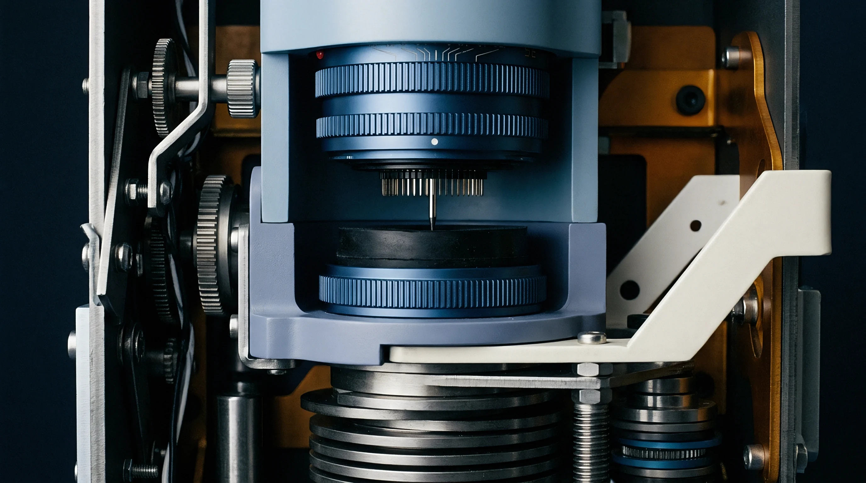
Jig
Calibration accuracy depends directly upon the physical stability and angular precision of mechanical positioning fixtures. Mechanical indexing mounts must hold the sensor package static in specific, known spatial orientations relative to the local earth gravity vector. Local gravity magnitude remains constant across short spatial distances, providing an absolute physical vector magnitude reference.
Spatial positioning deviations introduce systematic velocity and tilt errors into the mathematical solver.
Multi-axis indexing heads allow system operators to rotate sensors through precise angular increments. Mechanical dividers must provide repeatability below five arcseconds to prevent fixture position uncertainty from dominating the residual calibration error budget. Optical encoders mounted directly to rotation shafts verify orientation angles during automated calibration runs.
Mounting plates require high flexural rigidity to resist mechanical deflection caused by cable tension or temperature changes inside test chambers.

Orientation Schedules for Static Gravitational Vector Reference
Field calibration procedures employ discrete multi-position orientation schedules to isolate individual matrix parameters. Six-position tumble tests align each physical face of a rectangular test housing perpendicular to the earth surface, placing each sensing axis parallel and antiparallel to the static gravity vector. Six-position schedules expose primary zero-g offset biases and main diagonal scale factors with minimal computational overhead.
Complex orientation schedules increase parameter observability. Twelve-position schemes add forty-five-degree tilt steps between major orthogonal planes, exposing off-diagonal cross-axis misalignment terms. Twenty-four-position schedules distribute orientation vectors evenly across a spherical surface.
Increasing position counts reduces solver sensitivity to random measurement noise while averaging out localized mechanical mounting chatter.
| Orientation Schedule | Position Count | Observability Range | Execution Time per Unit | Target Residual Bias Noise |
|---|---|---|---|---|
| Cube Face Tumble | 6 Positions | Bias, Primary Scale Factors | 45 Seconds | 0.8 mg |
| Face and Edge Indexing | 12 Positions | Bias, Scale Factors, Cross-Axis Angles | 120 Seconds | 0.3 mg |
| Uniform Sphere Sampling | 24 Positions | Full 12-Parameter Matrix, Non-Linearity | 300 Seconds | 0.1 mg |
| Continuous Gimbal Rotation | Dynamic Sweep | Full Matrix, Centripetal Decoupling | 180 Seconds | 0.15 mg |
Static acquisition phases demand strict settling time enforcement. Sensor mechanical structures and digital anti-aliasing filters exhibit transient response delays following physical movement. Logging data prior to complete mechanical stabilization introduces motion-induced dynamic acceleration vectors into static gravity calculations.
Settling windows must exceed five times the combined mechanical resonance period and digital filter latency.

Tumble Fixture Mechanical Tolerances and Indexing Deviations
Indexing deviations introduce systematic leakage. Fixture surface non-planarity forces orthogonal positioning axes away from true vertical alignment ~ an indexing surface error of one milliradian transfers one millig-unit of vertical gravitational force directly into transverse measurement channels. Alignment errors corrupt cross-axis matrix calculations, causing calibration algorithms to generate false non-orthogonality correction factors.
Coordinate transformation matrices map sensor internal mechanical coordinates to fixture reference planes. Precision locating pins isolate package rotational mounting variances on printed circuit boards. Automated calibration benches utilize pneumatic clamping systems to maintain constant holding force without distorting thin-walled circuit board substrates.
Thermal isolation blocks prevent drive motor heat from flowing into test fixtures during long-duration automated calibration sequences.
Factory laser trimming covers baseline consumer requirements, but board-level reflow assembly generates severe mechanical stress across thermal profiles. Surface-mount reflow cooling contracts circuit board copper traces, transferring parasitic mechanical strain through package leadframes directly into silicon sensor dies and shifting factory offset calibrations entirely out of tolerance.

Matrix
Mathematical solvers extract calibration parameters by matching measured raw acceleration vectors to the invariant earth gravity magnitude. Under pure static conditions, the vector norm of true physical acceleration equals exactly one local earth gravity unit regardless of sensor orientation. Quadrated signal outputs plotted across all possible spatial directions trace out a deformed three-dimensional ellipsoid in raw measurement count space.
Ellipsoid parameter mapping converts physical distortion parameters into concrete linear algebra representations. An uncalibrated sensor yields an ellipsoid whose center offset corresponds to the zero-g bias vector. Axis elongation along coordinate directions reflects scale factor variations.
Spatial rotation and skewness of the ellipsoid axes represent non-orthogonality alignment angles and cross-axis coupling ratios. Parameter extraction routines solve for the matrix transformation that compresses and translates this deformed raw ellipsoid back into a perfectly centered unit sphere.

Ellipsoid Surface Fitting and Non Linear Least Squares Mechanics
Non-linear least squares algorithms minimize scalar residuals between reconstructed acceleration vector magnitudes and the local gravity reference constant. Define the scalar objective cost function across N discrete orientation measurements as:
J(M, b) = ∑ 2
Iterative optimization schemes like Gauss-Newton or Levenberg-Marquardt compute parameter updates by calculating partial derivative Jacobian matrices at each iteration step. Gauss-Newton steps update parameter estimate vectors by solving normal matrix equations based on local gradient vectors. Convergence relies upon initial parameter estimates remaining close to physical truth.
Properly executed ellipsoid surface fitting routines converge within six numerical iterations when initialized with unit scale factors and zero initial bias vectors.
Algebraic sphere fitting offers closed-form parameter generation without requiring iterative convergence loops. Algebraic methods formulate constraint equations into implicit quadratic surface forms solved directly via singular value decomposition. Algebraic fits process faster in embedded factory test setups but exhibit higher sensitivity to spatial measurement clustering compared to geometric distance minimization routines.
- Mount accelerometer securely into index fixture and initialize high-resolution raw count data collection at stable room temperature.
- Rotate fixture through prescribed orientation schedule, holding unit motionless at each position for two full seconds.
- Compute temporal mean raw count vectors for each static position to suppress white Gaussian measurement noise.
- Construct design matrix from raw mean count vectors and evaluate initial algebraic matrix estimates via singular value decomposition.
- Execute Gauss-Newton iterative refinement loop until objective cost parameter change drops below one part per million.
- Extract inverted scale factor transformation matrix and zero-g bias vector from final optimized surface equations.

Comparing Six Parameter and Twelve Parameter Mathematical Formulations
Reduced six-parameter correction models compute only three scalar biases and three primary scale factors. Six-parameter schemes assume perfect ninety-degree intersections between sensor internal coordinate axes. This simplified formulation eliminates matrix inversions, requiring only basic scalar subtraction and multiplication operations in target embedded microcontrollers.
Six-parameter models work adequately when cross-axis sensitivity specifications remain below zero point two percent.
Full twelve-parameter models compute three bias terms, three primary scale factors, and six independent cross-axis coupling parameters. Twelve-parameter formulations fully reconstruct arbitrary affine transformations, absorbing both internal die misalignment and circuit board mounting tilt. High-precision tilt measurement and dead-reckoning navigation systems mandate full twelve-parameter matrix correction to maintain long-term position integration stability.
| Model Formulation | Parameter Count | Cross-Axis Coupling | Floating-Point Operations per Sample | Residual Tilt Error |
|---|---|---|---|---|
| Offset Only | 3 Parameters | Ignored | 3 Subtractions | 1.85 deg |
| Diagonal Scale and Offset | 6 Parameters | Ignored | 3 Subtractions, 3 Multiplications | 0.42 deg |
| Orthogonal Scale and Offset | 9 Parameters | Symmetric Model | 3 Subtractions, 9 Multiplications | 0.08 deg |
| Full Affine Transformation | 12 Parameters | Asymmetric Model | 3 Subtractions, 9 Multiplications, 6 Additions | 0.01 deg |
Matrix invertibility dictates algorithm stability during real-time embedded compensation execution. Singular value decomposition checks identify ill-conditioned transformation matrices resulting from poor orientation coverage. Calibration schedules that fail to span all three dimensional axes yield rank-deficient design matrices that generate unstable correction parameters.
Calibration parameter accuracy scales directly with spatial sample distribution density across all spatial octants.

Drift
Temperature fluctuations alter the physical geometry and mechanical stresses within silicon MEMS transducers. Silicon flexures soften as temperature rises, decreasing internal mechanical resonant frequencies. Material thermal expansion coefficient mismatches between silicon substrates, glass frit bonding layers, and organic circuit board materials generate temperature-dependent mechanical forces.
Mechanical expansion shifts internal sensing comb structures, producing significant thermal offset drift and scale factor variation.
Thermal offset drift coefficients quantify zero-g output shifts across temperature variations. High-grade industrial sensors exhibit offset drift rates between zero point one and zero point five millig-units per degree Celsius. Uncompensated thermal drift causes static tilt calculations to wander over ambient operational cycles.
Linear temperature coefficients fail to model non-linear thermal stress behavior observed across extended automotive operating temperature bands.

Thermal Soak Schedules and Multi Temperature Vector Solves
Thermal chamber calibration executes orientation tumble schedules across multiple discrete temperature setpoints. Environmental test chambers ramp ambient temperatures across target operational ranges while maintaining strict thermal stability controls. Thermal soak enforcing structural stability prevents spatial temperature gradients across the sensor package from corrupting static measurement data.
Internal temperature sensors embedded directly on the silicon die provide true junction temperature references.
Multi-temperature vector extraction routines process static tumble data gathered at each discrete temperature step. The calibration system computes independent twelve-parameter calibration matrices for each temperature soak plateau. Linking extracted parameters to die temperature measurements forms discrete parameter sequences that characterize environmental sensor behavior across the entire operational envelope.
IEEE standard 1431 section eight specifies that environmental sensor calibration thermal equilibrium requires temperature rates of change below zero point zero five degrees Celsius per minute prior to data logging.
Polynomial curve fitting constructs continuous temperature-dependent correction models from discrete thermal matrix evaluations. Quadratic and cubic polynomial functions model zero-g bias and scale factor variation as functions of die junction temperature. Higher-order polynomial terms track non-linear thermal expansion effects occurring at extreme temperature limits.
- Temperature Coefficient of Offset measures the linear shift in zero-g output bias per unit change in die temperature.
- Temperature Coefficient of Sensitivity tracks the percentage change in channel gain per degree Celsius variation from reference calibration temperatures.
- Thermal Soak Settling Window enforces adequate dwell time at target temperatures to eliminate internal component thermal gradients.
- Package Thermal Hysteresis captures path-dependent measurement shifts occurring when approaching target temperatures from opposite thermal directions.
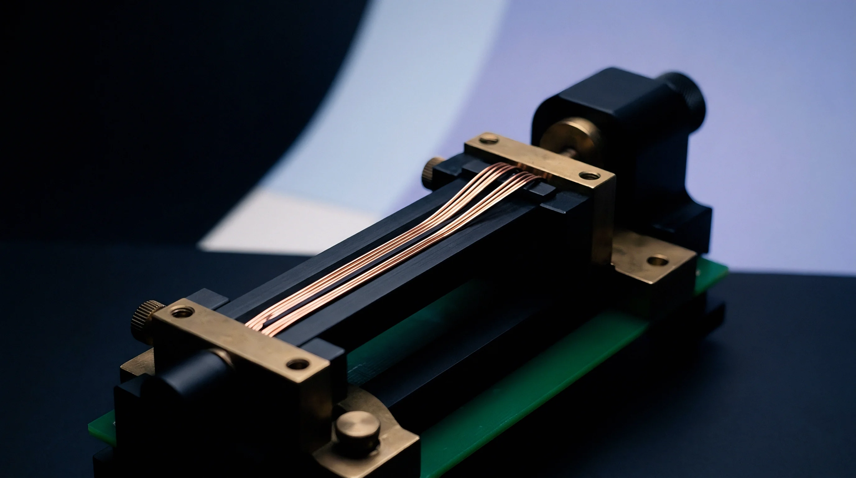
Why Does Thermal Hysteresis Defeat Static Polynomial Correction?
Package thermal hysteresis introduces path-dependent offset deviations that simple polynomial functions cannot model. Internal plastic encapsulation materials absorb moisture and experience structural stress relaxation during thermal cycling. Cooling a sensor from hot extremes produces different internal mechanical strain fields than heating the same sensor from sub-zero conditions.
The resulting zero-g offset curves form closed hysteresis loops across thermal cycles.
Dual-path polynomial models track heating and cooling phases independently by monitoring internal die temperature rates of change. System firmware evaluates the temporal derivative of die temperature to select appropriate heating or cooling polynomial matrix coefficients. Incorporating thermal rate tracking suppresses hysteresis-induced zero-g offset uncertainty by more than sixty-five percent during rapid ambient temperature shifts.
| Compensation Strategy | Polynomial Order | Temperature Band | Peak Offset Drift | Memory Footprint |
|---|---|---|---|---|
| Uncompensated Baseline | None | -40 deg C to +85 deg C | 28.5 mg | 0 Bytes |
| Linear Polynomial Fit | 1st Order | -40 deg C to +85 deg C | 4.2 mg | 24 Bytes |
| Quadratic Polynomial Fit | 2nd Order | -40 deg C to +85 deg C | 1.1 mg | 48 Bytes |
| Hysteresis Dual-Path Model | 2nd Order + Derivative | -40 deg C to +85 deg C | 0.3 mg | 96 Bytes |
ISO standard 16063 section sixteen mandates that primary vibration and gravity calibration records explicitly document environmental temperature stability bounds alongside reported sensor measurement uncertainties. Contracts that omit operational thermal stability clauses leave component buyers fully exposed when field units experience thermal drift failures under extreme operational environments.

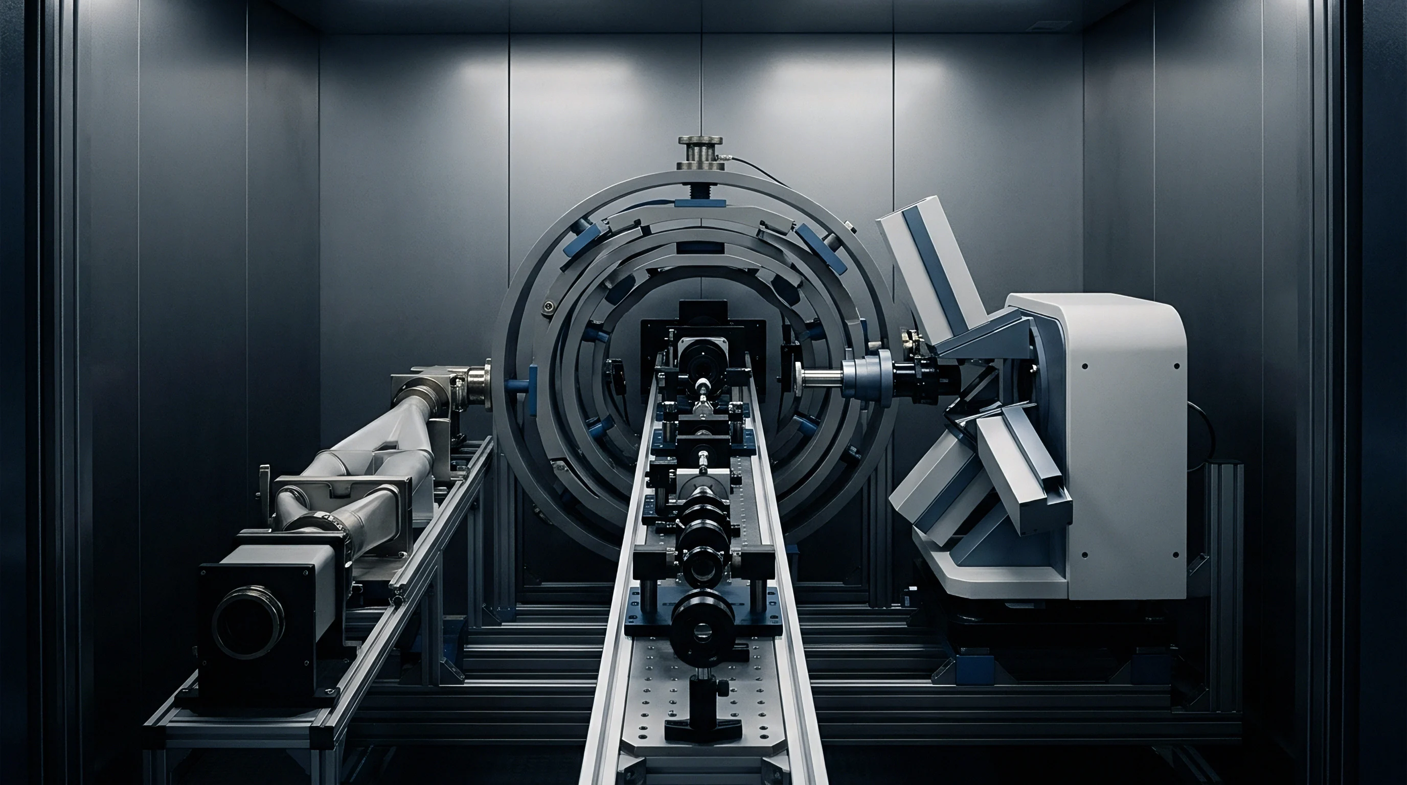
Proof
Verification metrics evaluate post-calibration vector accuracy by comparing reconstructed acceleration magnitudes to known physical gravity references. Residual acceleration variance serves as the primary statistical metric for calibration quality assessment. The scalar residual norm error for a specific orientation evaluation is calculated as:
ei = || M-1 · ( yi – b ) || – glocal
Root mean square error calculations aggregate scalar residual norm errors across all test orientations. Achieving root mean square residual values below zero point two millig-units confirms successful parameter optimization and effective noise suppression. Residual plots that exhibit spatial correlation patterns indicate uncompensated non-linearities or mechanical fixture indexing errors.

Residual Acceleration Variance and Verification Metrics
Assessing performance demands testing calibrated accelerometers at spatial orientations entirely independent of the original calibration schedule angles to confirm parameter fit. Evaluating vector outputs across arbitrary three-dimensional tilt positions validates matrix generalization across real-world operational profiles. Systems that display low residuals at calibration points but high errors at intermediate positions suffer from parameter over-fitting.
Angular tilt error calculations convert residual acceleration norm errors into concrete angular inclination uncertainties. Static tilt angle error maps directly to residual acceleration through the small-angle approximation equation:
θerr ≈ erms / glocal
A residual acceleration error of zero point5 millig-units translates directly into a static inclination error of approximately zero point zero two nine degrees. High-precision leveling systems requirement specifications bound total allowable angular error, establishing strict upper limits for acceptable residual acceleration variance following static calibration routines.
| Performance Metric | Raw Sensor Output | 6-Parameter Calibrated | 12-Parameter Calibrated |
|---|---|---|---|
| Vector Norm Variance | 42.5 mg | 3.8 mg | 0.18 mg |
| Static Inclination Precision | 2.43 deg | 0.22 deg | 0.01 deg |
| Axis Cross-Talk Ratio | -28 dB | -42 dB | -65 dB |
| Long-Term Bias Stability | 12.0 mg/yr | 1.5 mg/yr | 0.4 mg/yr |
Fixed point rounding introduces quantization noise inside low-power microcontrollers during online matrix multiplication routines.
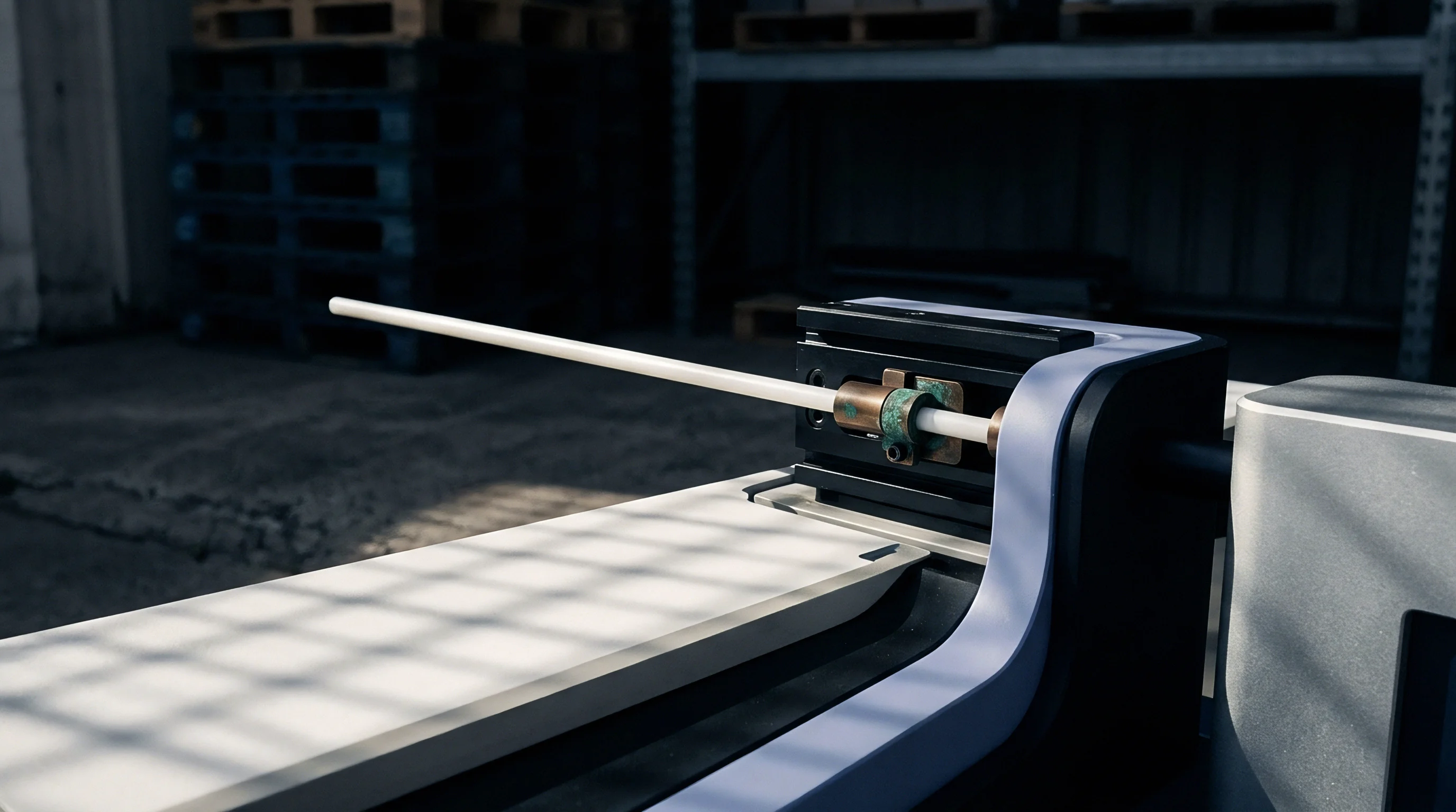
Fixed Point Mathematical Execution in Embedded Controllers
Embedded microcontrollers execute parameter compensation in real-time within primary sensor interrupt service routines. Floating-point units execute twelve-parameter matrix compensation rapidly but consume significant active power. Low-power internet-of-things edge nodes utilize integer fixed-point arithmetic to process matrix equations without waking floating-point hardware extensions.
Fixed-point scale factor representation requires careful binary point allocation to prevent numerical overflow and underflow conditions. Scale factors stored as thirty-two-bit signed integers with sixteen fractional bits maintain numerical precision across wide gain adjustment ranges. Matrix multiplication algorithms accumulate intermediate products inside sixty-four-bit registers prior to bit-shifting operations to prevent truncation noise from degrading calibrated measurement resolution.
Static twelve-parameter transformation pipelines operating on integer fixed-point math consume less than two hundred clock cycles per triaxial conversion step on standard ARM Cortex-M microcontrollers.
Memory allocations store twelve transformation parameters alongside temperature polynomial coefficients inside non-volatile EEPROM or flash memory regions. Microcontroller boot sequences load calibration parameters into system RAM structures during system initialization. Integrity checksums verify parameter block flash memory contents prior to enabling active sensor measurement channels.
Whether embedded multi-temperature vector calibration matrixes can dynamically adapt to decade-long structural adhesive creep inside sealed automotive sensor housings remains an open question.