Quantifying Multi Node Observer State Drift under Temperature Dependent Transducer Matrix Parameter Variance in Embedded Field Deployments
Thermal gradients induce unmodeled transducer matrix parameter shifts that destabilize multi-node observers unless decoupled via polynomial pre-inversion.

Gradient
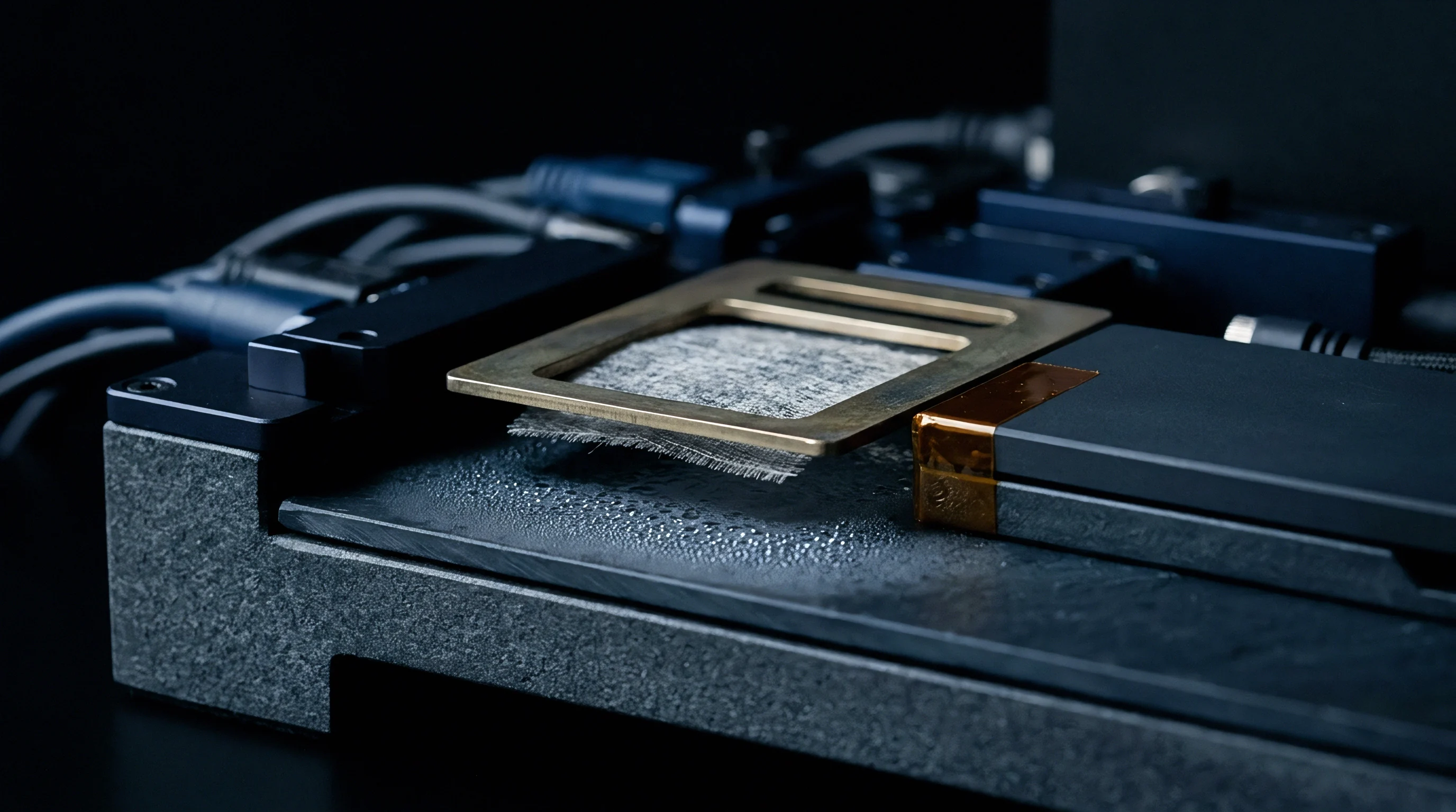
Thermal gradients across distributed sensing layouts destabilize observer state estimates long before individual transducer elements reach their datasheet operating limits. In a multi-node estimator like an extended Kalman filter or distributed consensus architecture, parameter variance is assumed to follow the spatial or temporal distribution declared during calibration. When ambient temperature swings induce unmodeled divergence across local nodes, state drift accumulates through the network topology.
Transducer elements exposed to uneven solar loading, varying convection currents, or localized power dissipation undergo asymmetric changes in sensitivity, bias, and cross-axis alignment. The math behind the observer attributes these sensor variations to actual changes in the asset being monitored.
Differential temperatures alter transducer transfer functions across nodes at distinct rates. A localized junction temperature difference of 15 degrees Celsius between two sensing nodes running identical piezoresistive pressure cells produces an uncalibrated sensitivity mismatch exceeding 0.3 percent of full scale. The observer treats that response as a real spatial gradient across the physical process.
Left uncorrected, the internal covariance matrices of the estimator misalign with real measurement errors. Filter gains fail to damp the divergent readings, and the network state estimate drifts away from physical ground truth.
Direct mathematical quantification of this divergence demands an explicit split between process noise and observation matrix variance induced by thermal sensitivity coefficients. Rather than relying on a static measurement matrix, the observer architecture has to account for parameter variance in each transducer element across operational temperature spans.
Commercial piezoresistive transducer arrays demonstrate span temperature coefficients shifting between minus 0.15 and minus 0.22 percent per degree Celsius without external conditioning.
Establishing baseline stability requires mapping the temperature coefficient of sensitivity alongside zero-offset thermal drift for each transducer modality deployed across the structural nodes.
- Sensitivity temperature drift alters the gain matrix directly, scaling the measurement vector proportionally with ambient variance.
- Zero offset thermal shift injects additive measurement bias into individual node observers, masquerading as low-frequency process dynamics.
- Axis alignment deviation emerges from mismatched thermal expansion coefficients within mechanical packaging, rotating the transducer matrix relative to the local reference frame.
- Transconductance temperature decay diminishes the effective resolution of piezoresistive and capacitive conditioning circuits, elevating the node noise floor.
Quantifying these shifts across a field deployment reveals whether an apparent multi-node state fluctuation originates in the measured medium or within the mounting fixtures of the instrument array.

Coupling
Thermal coupling between structural enclosures and internal transducer dies governs how fast environmental swings shift internal measurement matrices. Transducers housed in aluminum field enclosures exhibit rapid thermal tracking, whereas units seated on thermal isolation standoffs encounter steep internal gradients between the external process fluid interface and the signal-conditioning substrate. That physical interaction dictates how the observation matrix must be constructed.
For an observer state vector tracking physical spatial coordinates, velocities, or process pressures, the discrete-time linear observation equation links the true state vector to the measurement vector through the transducer observation matrix. When temperature varies across node locations, this observation matrix shifts away from nominal calibrated values.
In a standard three-axis measurement node tracking state through three orthogonal transducers, the nominal matrix reflects unit sensitivity along principal axes with zero cross-axis coupling. But as thermal stress acts on the die attach and package leadframe, asymmetric mechanical deformation rotates the sensing elements. A temperature divergence of 40 degrees Celsius away from calibration shifts the off-diagonal terms of the matrix through mechanical stress coupling.
Package-induced die stress under thermal cycling rotates the off-axis sensitivity coefficients by up to 0.012 per 100 degrees Celsius in molded plastic packages.
The resulting deviation between nominal and physical transducer behavior feeds observation errors straight into the state update sequence. Update equations calculate an innovation vector representing the discrepancy between actual measurements and predicted states. When the transducer matrix varies with temperature, the innovation vector carries a persistent, non-zero bias that the estimator mistakes for a driving disturbance within the physical process itself.
Integrating thermal models into the observer parameterizes the transducer matrix as a function of measured local board temperatures. If the temperature sensor on the conditioning board lags the physical transducer die by a significant thermal time constant, dynamic temperature changes break the tracking loop. The resulting lag induces transient state drift that persists until the assembly settles into thermal equilibrium.
| Transducer Principle | Parameter Shift Coefficient | Test Condition | Observer Innovation Error | Primary Mechanism |
|---|---|---|---|---|
| Silicon Piezoresistive | Minus 0.18 percent per Kelvin | Constant Current, 25 to 85 C | 1.45 percent of span | Piezoresistive coefficient decay |
| Capacitive MEMS | Plus 35 parts per million per Kelvin | Constant Voltage, minus 40 to 85 C | 0.28 percent of span | Electrode gap thermal expansion |
| Thin-Film Strain Gauge | Plus 0.008 percent per Kelvin | Wheatstone Bridge, 20 to 100 C | 0.06 percent of span | Substrate expansion mismatch |
| Bulk Piezoelectric | Minus 0.04 percent per Kelvin | Charge Amplifier, 20 to 120 C | 0.32 percent of span | Curie temperature proximity loss |
Designing embedded field deployments involves matching physical transducer time constants to the digital estimator tracking speed to suppress dynamic observer divergence.
Divergence
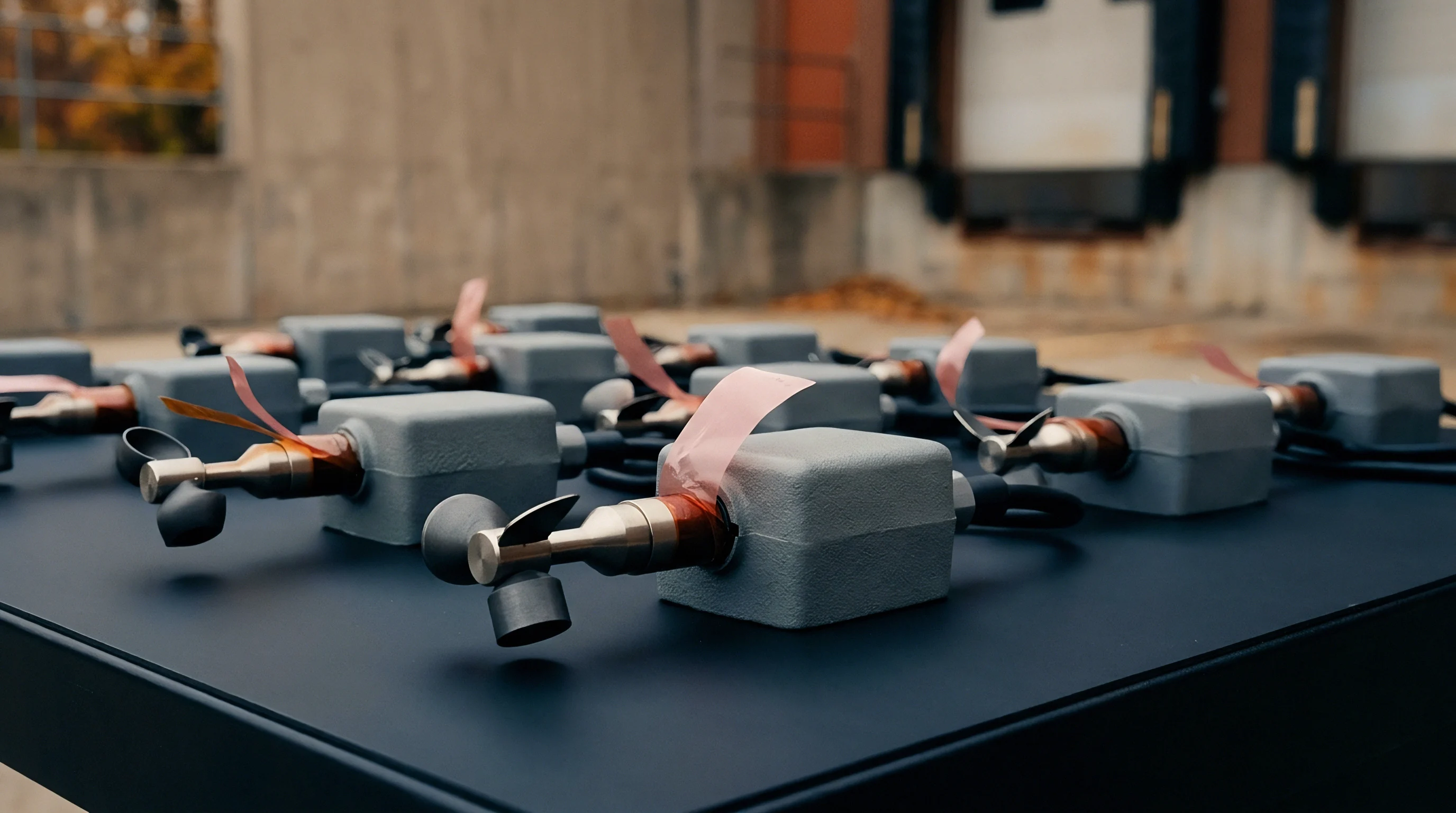
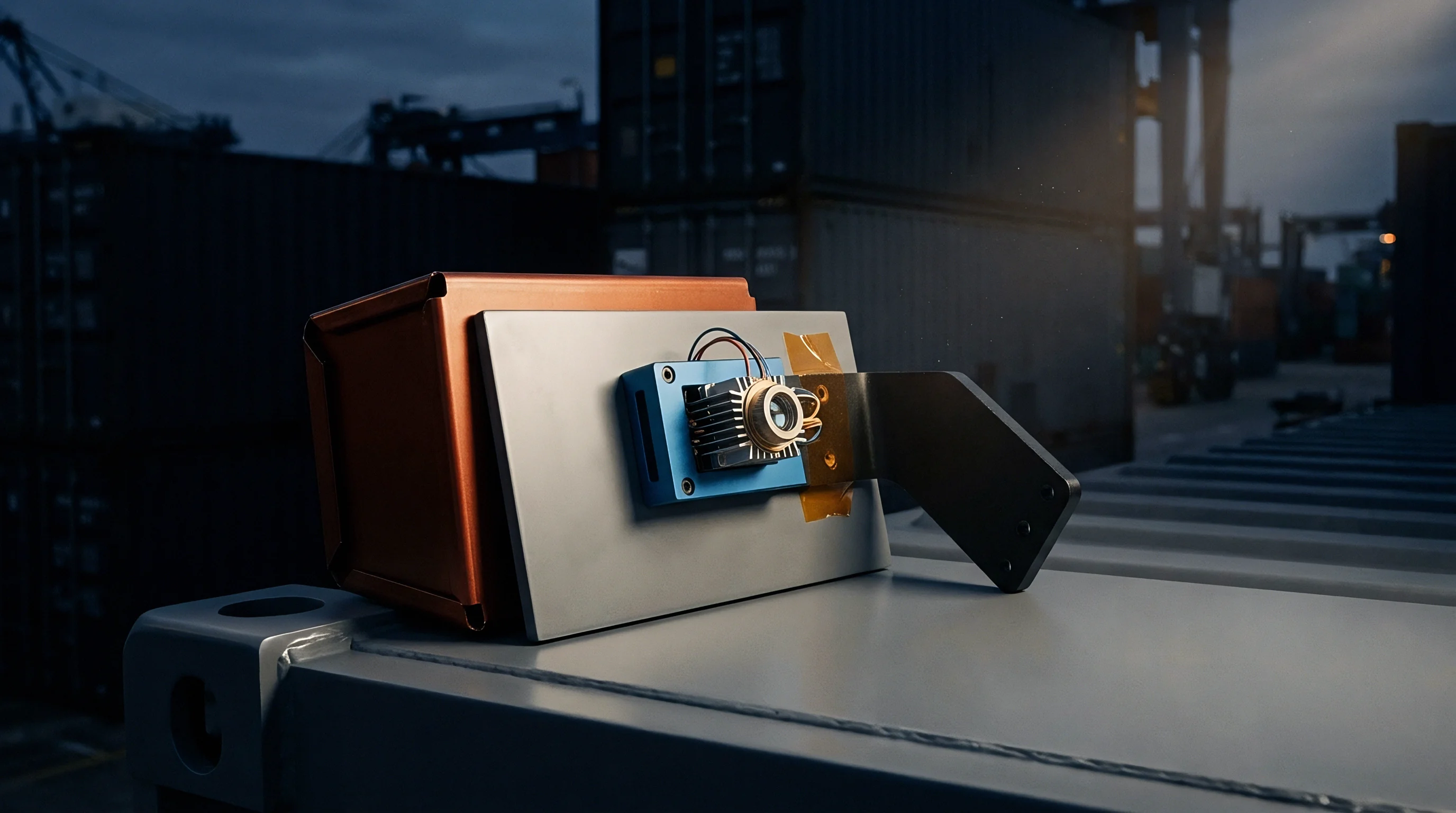
Quantifying multi-node observer drift mathematically requires calculating how bounded parameter errors propagate into unbounded state variance. When multiple nodes report state estimations to a central consensus filter, cross-node variance in transducer parameters creates spatial dissonance: the central observer can no longer distinguish between a traveling mechanical wave, an uneven process distribution, or localized thermal drift.

Observer Stability Limits
The discrete Kalman filter state estimation error covariance matrix evolves according to the Riccati equation. When the observation matrix deviates from its calibrated model by an error matrix, the actual estimation error covariance departs from the computed error covariance. The filter assumes its confidence bounds are narrow while actual state error expands unchecked.
In localized deployments, whenever the error matrix norm exceeds the ratio of process noise covariance to measurement noise covariance, positive feedback drives states toward divergence.
Spatial Covariance Degradation
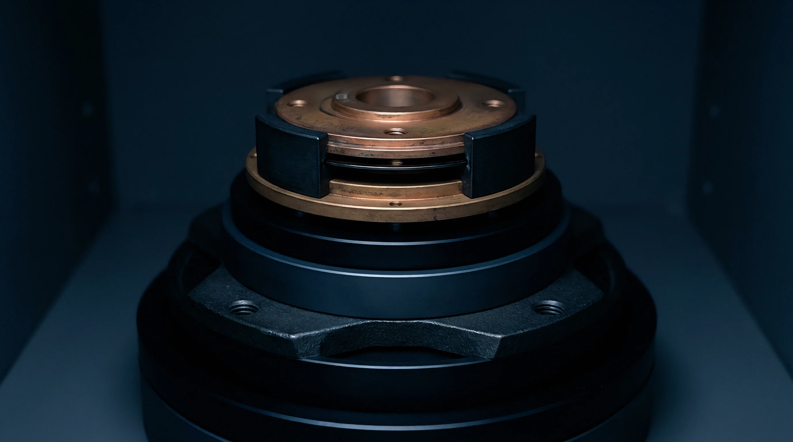
Multi-node topologies rely on spatial correlations to validate measurements across neighboring units. Take an eight-node array deployed along a pipeline structure: if four nodes sit in direct sunlight at 48 degrees Celsius and four shaded nodes rest at 28 degrees Celsius, the sunlit nodes report lower signal amplitudes due to the negative temperature coefficient of sensitivity in their piezoresistive cores.
The spatial consensus algorithm attempts to reconcile these differing values. Because the observer treats all nodes as identical instruments operating under symmetric noise distributions, it pulls the overall network state toward an artificial middle ground, computing false gradient vectors across the physical structure.
A temperature divergence of 20 Kelvin across nodes causes multi-node observer convergence errors exceeding four times the single-node measurement noise floor.
Calculating the exact drift bound requires modeling parameter variance as a bounded perturbation matrix. Applying Lyapunov stability criteria to the error system yields an upper bound on steady-state estimation error. If the thermal compensation loop fails to maintain parameter divergence below a calculated critical threshold, the entire distributed state network forfeits mathematical convergence.
Field data confirms that neglecting this cross-node parameter variance leads to phantom alarms and false actuator adjustments triggered by the control automation layer.
Drift
Tracing the true drift trajectory involves setting up an analytical sequence across embedded compute cycles. The following numerical derivation illustrates how thermal variance transforms nominal sensor outputs into escalating state error over a standard operational cycle.
Step by Step Parameter Matrix Derivation
Take an embedded array of three structural strain monitoring nodes positioned around a turbine housing. Each node samples a three-dimensional stress state using a triaxial resistive gauge array. The nominal transducer matrix is an identity matrix scaled by a conversion gain of 2.0 millivolts per microstrain at a baseline calibration temperature of 20 degrees Celsius.
The nodes run localized discrete Kalman observers tracking mechanical deflection.
During an operational cycle, temperature logs register Node 1 at 35 degrees Celsius, Node 2 at 55 degrees Celsius, and Node 3 at 75 degrees Celsius. The thin-film gauge exhibits a sensitivity temperature coefficient of plus 0.015 percent per degree Celsius and an offset drift coefficient of plus 1.2 microstrain per degree Celsius. Meanwhile, anisotropic thermal expansion of the structural mounting block introduces off-axis cross-coupling equal to 0.0004 per degree Celsius above baseline.
- Baseline parameter calculation establishes the nominal gain matrix at 20 degrees Celsius with zero offset across all three axes.
- Thermal delta calculation isolates temperature variations of 15 Kelvin for Node 1, 35 Kelvin for Node 2, and 55 Kelvin for Node 3.
- Matrix perturbation mapping applies the combined sensitivity and cross-coupling shifts to populate the individual transducer observation matrices.
- State innovation calculation multiplies the perturbed measurement matrices by the actual mechanical strain vector of 500 microstrain along the primary axis.
- Residual accumulation assessment tracks the observer state vector as the Kalman gain integrates the unmodeled measurement delta across 1000 update intervals.
Node 3 experiences a sensitivity gain shift of plus 0.825 percent and an additive offset bias of 66 microstrain, with off-axis matrix terms rising from 0.0 to 0.022. Multiplying this perturbed matrix by the 500 microstrain mechanical vector yields an apparent output of 570.1 microstrain on the primary axis, with an erroneous 11.0 microstrain coupled into the orthogonal axes.
The localized Kalman observer calculates an innovation residual of 70.1 microstrain. Over 1000 discrete update cycles with a Kalman gain factor of 0.05, the uncorrected observer pushes the estimated deflection state upward by 68.3 microstrain above true mechanical reality, attributing deformation to the turbine shell when the asset remains structurally unchanged.
When the central multi-node fusion engine executes its spatial correlation check, the discrepancy between Node 1 (reporting 518.5 microstrain) and Node 3 (reporting 568.3 microstrain) triggers a false structural twist warning. The quantitative divergence derives entirely from transducer parameter shifts rather than physical movement.

Compensation
Mitigating multi-node observer drift requires active algorithmic and hardware compensation strategies implemented directly at the embedded edge. Modifying firmware to account for real-time thermal variance stabilizes the observer without demanding costly mechanical thermal regulation across the field deployment.

Why Not Augment the Observer State Vector Directly?
Augmenting the observer state vector with transducer calibration parameters appears mathematically direct: by appending sensitivity and bias terms to the state vector, an extended Kalman filter attempts to estimate both physical system state and transducer calibration shifts simultaneously. In embedded field nodes, this approach degrades computational stability because the system matrix loses local observability when process input excitations drop to zero.
If an asset enters a steady-state dwell period where stress, pressure, or motion does not fluctuate, the observer cannot distinguish between offset drift in the transducer die and low-frequency drift in the monitored asset. Appending these extra parameters doubles the covariance matrix dimension, multiplying execution cycle times by four. Embedded microcontrollers with constrained floating-point units face execution timing violations or truncation errors that destabilize numerical integration routines.

Polynomial Matrix Realignment
A preferred strategy implements decoupled polynomial correction prior to the observer innovation stage. Each transducer node runs an internal temperature measurement channel situated adjacent to the sensing element. During factory calibration, the transducer array is characterized inside an environmental chamber across its operating span from minus 40 to plus 105 degrees Celsius, generating a temperature-dependent inverse correction matrix.
| Correction Strategy | Computational Complexity | Observer Stability | Residual State Drift | Memory Footprint |
|---|---|---|---|---|
| Augmented State EKF | High: cubic scaling with state count | Marginal under static input dwell | 0.8 to 1.2 percent full scale | 14.2 kilobytes RAM |
| Polynomial Pre-Inversion | Low: quadratic scaling with order | High across all operational profiles | 0.05 to 0.12 percent full scale | 1.8 kilobytes RAM |
| Online Covariance Inflation | Moderate: linear matrix updates | High: preserves asymptotic bounds | 0.4 to 0.7 percent full scale | 3.4 kilobytes RAM |
| Consensus Gradient Balancing | High: requires inter-node telemetry | Medium: dependent on communication lag | 0.15 to 0.30 percent full scale | 8.6 kilobytes RAM |
The polynomial pre-inversion method normalizes incoming measurements before they enter the observer innovation calculation. The observation matrix remains constant, preserving the computational efficiency of the steady-state gain calculation while eliminating the root cause of state divergence.
Standard procurement specifications for sensor performance must include maximum allowable thermal hysteresis along with sensitivity drift bounds to ensure the validity of these polynomial pre-inversion matrices over multi-year field operations.

Yield
Procuring transducer arrays capable of maintaining multi-node observer stability requires assessing factory test methodology and batch-level parameter distribution. Transducer specifications routinely quote typical temperature coefficients derived from a small sample set measured at nominal supply voltages. In mass production, semiconductor doping variations, micromachined membrane thickness deviations, and leadframe alloy tolerances generate substantial spreads in sensitivity temperature coefficients.
A component lot exhibiting a nominal sensitivity temperature coefficient of minus 0.15 percent per degree Celsius often spans a range from minus 0.08 to minus 0.24 percent across a single production wafer. When two transducers from opposite tails of this distribution land in the same multi-node array, their differential thermal response exceeds the compensation limits of factory default firmware. The multi-node observer diverges under thermal cycling even though every individual sensor functions within catalog parameters.
A four-point factory temperature calibration across production lots adds 3.20 dollars per unit to baseline transducer landed costs.
Protecting multi-node observer integrity requires explicit incoming inspection procedures to classify and group transducers by thermal drift signatures before field assembly. The qualification procedure evaluates baseline offset variance, gain temperature coefficient spread, and off-axis coupling shifts across simulated operational profiles in thermal chambers.
Neglecting this screening step shifts the engineering burden into complex firmware workarounds that lengthen validation timelines and drive up recurring field maintenance costs.


Audit
Verifying observer integrity under dynamic environmental stress demands rigorous field audit protocols executed after complete system assembly. Bench testing with precision power supplies and synthetic sensor inputs fails to capture the mechanical and thermal interactions that destabilize multi-node networks in real field enclosures.
Environmental Chamber Test Matrices
Field verification requires subjecting the entire multi-node instrumentation cluster to simultaneous thermal gradients and mechanical inputs. Test protocols specify thermal transition rates of up to 5 degrees Celsius per minute while monitoring the internal state variables of the distributed observer. Discrepancies between node internal state estimates and reference laser metrology or secondary laboratory instruments reveal the true scale of temperature-induced observer divergence.
Sensors are mounted to representative structural substrates to capture mechanical strain induced by mismatched coefficients of thermal expansion between the transducer packaging, the interface bracket, and the asset surface. This mechanical thermal coupling often overshadows internal die parameter shifts, injecting large unmodeled inputs into the observer array.
During the verification cycle, the test engineer records both raw transducer measurements and final filtered observer states to isolate where drift originates. An unstable observer exhibits growing innovation residuals alongside divergence between spatial node estimates, pointing toward inadequate parameter variance compensation in the observation equations.
The qualification dossier must document these drift metrics across the full environmental envelope defined in IEC 60068 standards before the hardware design passes into production release.
Unresolved questions persist regarding whether dynamic thermal gradients across high-density transducer arrays can be fully decoupled from physical asset deformation using purely mathematical compensation models without dedicated local reference heat sinks.