Modeling Non-Stationary Bias Drift across Thermal Gradients in Extended State Estimators for Tactical Sensors
Dynamic thermal gradients induce non-stationary bias drift in tactical sensors; state estimators must augment state vectors with thermal rate terms.
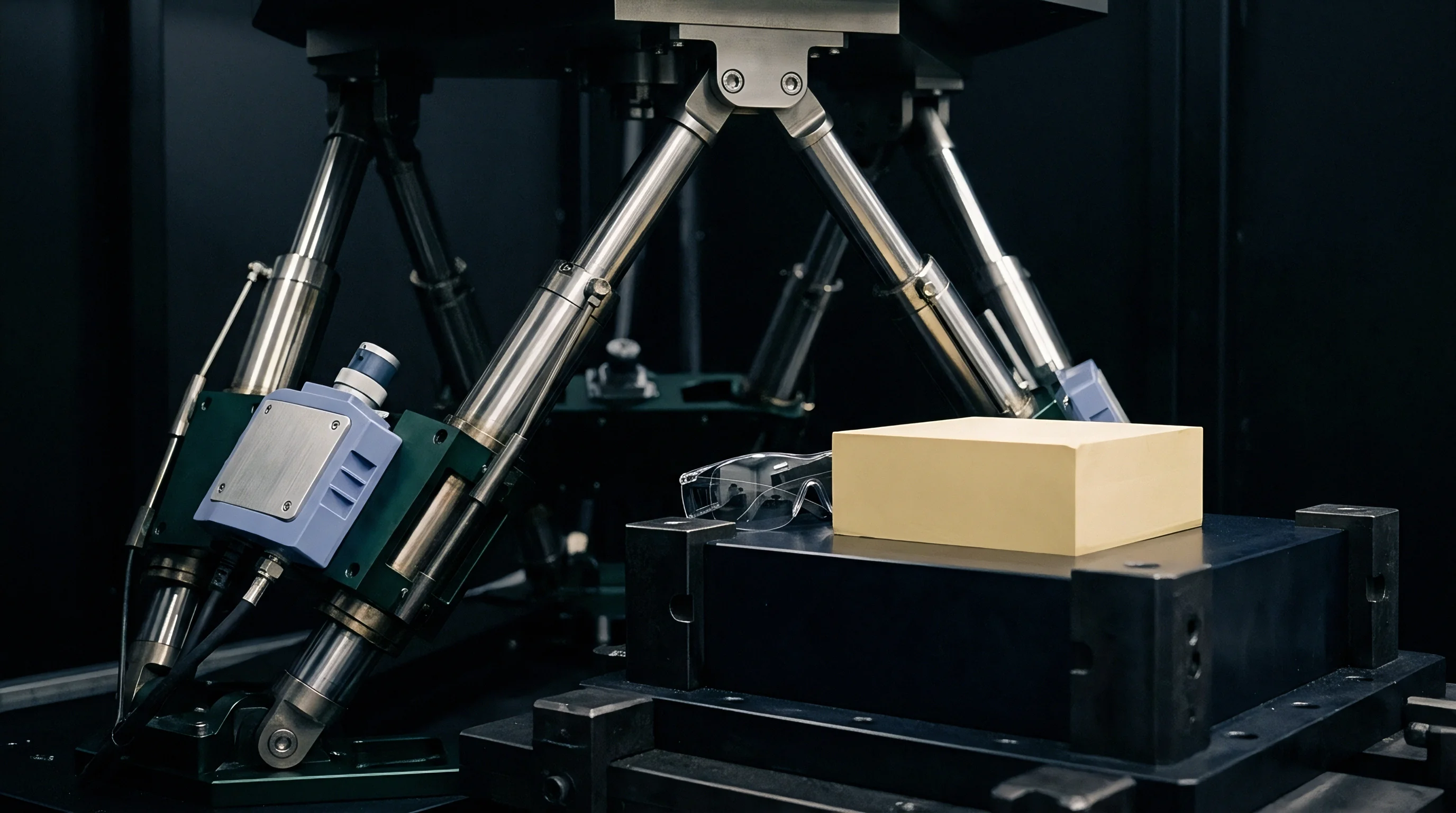
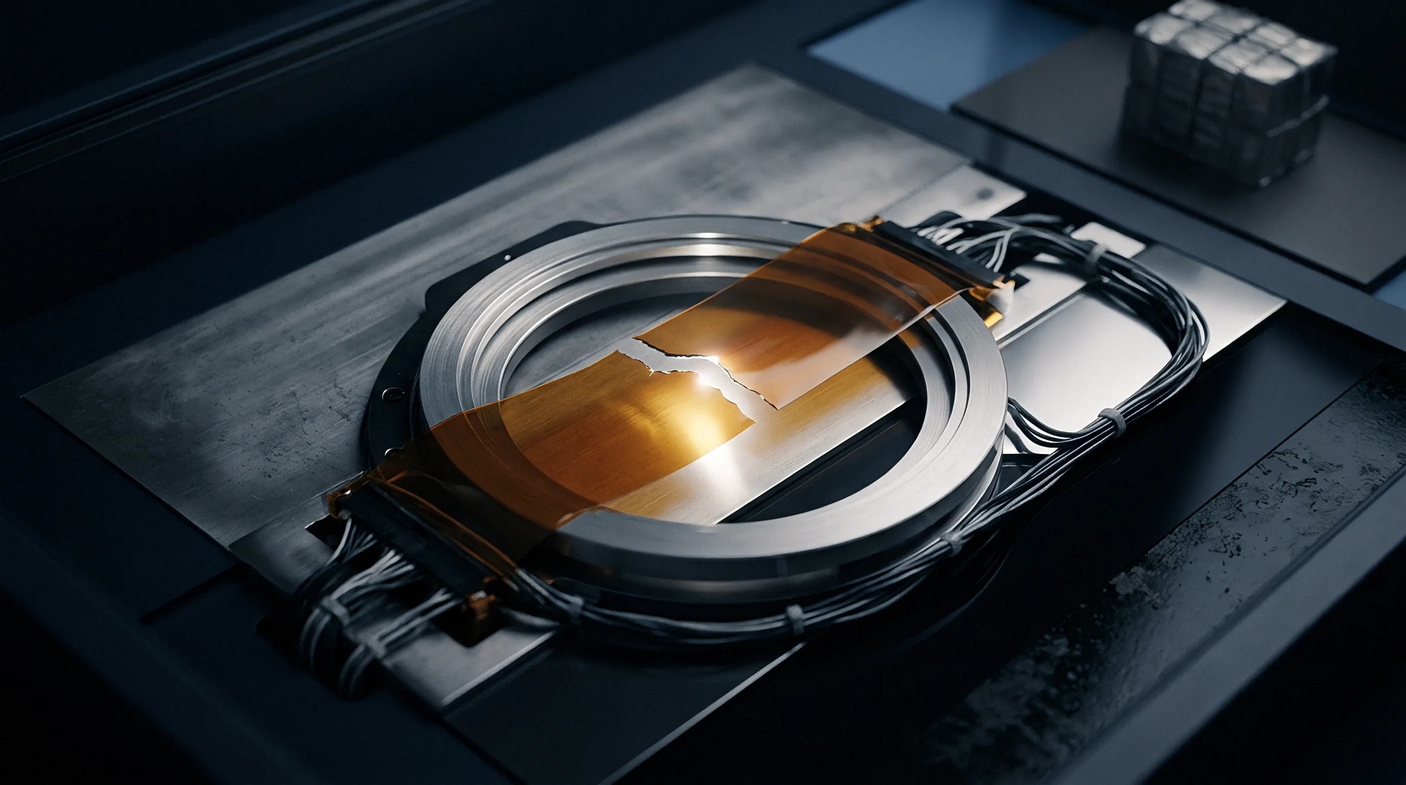
Heat
Temperature gradients across tactical-grade inertial sensors transfer localized energy that disrupts basic transduction mechanics. Rapid atmospheric shifts and internal power dissipation in guided projectiles, uncrewed aerial systems, and hypersonic re-entry vehicles cause steep, directional thermal shocks. Sensor components do not heat or cool uniformly.
Conduction through ceramic packaging, metal enclosures, and silicon substrates takes time, governed by each material’s diffusivity. When external temperatures swing faster than five degrees Celsius per minute, internal conduction lags, creating sharp spatial temperature differences across the sensing element.
Micro-electromechanical gyroscopes and accelerometers rely on sub-micron structural clearances to measure deflection through differential capacitance or piezoresistive strain, while fiber optic gyroscopes depend on symmetric optical path lengths within a wound coil. Dynamic heat flows break this physical symmetry. As heat moves inward from the housing, the frame expands locally before thermal changes reach the internal temperature sensor.
Because the temperature sensor on the readout integrated circuit sits on the periphery, its reading lags the actual temperature of the resonant mass or optical core. Standard calibration assumes thermal equilibrium ~ that die and housing temperatures match. During rapid thermal transients, that assumption breaks down, introducing unmodeled, non-stationary bias drift into the state estimator.
Heat diffusion through a solid body follows Fourier conduction dynamics, where thermal redistribution depends on material conductivity, density, and specific heat capacity. The characteristic thermal time constant dictates how quickly a structure returns to equilibrium after a temperature step:
tau_d = L^2 / alpha
Here, L is the physical distance between the package exterior and the transducer core, and alpha is the thermal diffusivity of the packaging stackup. Standard tactical MEMS architectures have thermal time constants from 12 to 45 seconds. Fiber optic gyroscope spools ~ with their larger mass and complex potting compounds ~ show time constants exceeding 180 seconds.
Across rapid thermal transients, gradients across the package frame drive structural deformation for the entire diffusion period.
| Sensory Transduction Principle | Package Material Stackup | Thermal Diffusivity alpha (m^2/s) | Characteristic Time Constant tau_d (s) | Uncompensated Drift Rate (deg/hr per deg C/min) |
|---|---|---|---|---|
| Silicon Capacitive Quad-Mass MEMS | LCC Ceramic on FR4 Substrate | 8.2 x 10^-6 | 14.2 | 1.85 |
| Piezoresistive Silicon Accelerometer | Kovar Lid on Alumina Substrate | 1.2 x 10^-5 | 9.8 | 0.42 milli-g per deg C/min |
| Quad-Symmetric Ring Resonant MEMS | Hermetic Titanium Package | 6.8 x 10^-6 | 28.5 | 0.65 |
| Closed-Loop Fiber Optic Gyroscope | Anodized Aluminum Chassis with Quad-Polar Fiber Wind | 1.4 x 10^-5 | 210.0 | 0.08 |
| Data taken under dynamic chamber thermal ramps between -40 degrees C and +85 degrees C at slewing rates of 5.0 degrees C/min without active state augmentation. | ||||
The lag between the sensing element’s actual temperature and the readout sensor’s measurement creates a dynamic phase delay. As heat moves inward, the package expands first, shifting structural preload on the mounting die before the readout thermistor registers any temperature change. Because of this phase mismatch, a single temperature reading can correspond to several different bias states depending on whether the unit is heating or cooling.
The relationship between temperature and bias ceases to be one-to-one, forming dynamic hysteresis loops.
In a tactical Extended Kalman Filter, unmodeled dynamic hysteresis acts as systematic measurement corruption. Estimators configured for stationary white process noise mistake these thermal bias shifts for real vehicle maneuvers or platform acceleration, incorrectly updating velocity and position states to track a false transient. Within ninety seconds of severe thermal slewing, position error variance grows exponentially, degrading target tracking accuracy.
Structural symmetry in sensing elements fails whenever internal thermal conduction rates lag external ambient thermal transitions.
Ignoring internal thermal transport physics in state estimator design leads to heavy estimation drift during engine ignition, rapid altitude shifts, or atmospheric re-entry. Once the estimator loses orientation accuracy, downstream guidance software issues false trajectory corrections that consume limited control margins.

Stress
Thermo-mechanical deformation in tactical transducers comes from mismatched thermal expansion coefficients among adjacent materials. An inertial measurement unit combines silicon sensing dies, glass frit bond layers, ceramic substrates, organic die-attach adhesives, and metallic enclosures. Silicon has an expansion coefficient near 2.6 x 10^-6 per Kelvin, alumina ceramic sits at 6.5 x 10^-6 per Kelvin, and copper traces reach 16.5 x 10^-6 per Kelvin.
When operational temperatures shift quickly, these mismatched expansion rates build mechanical shear strain across structural interfaces.
Shear strain distorts resonant structures, comb-finger gaps, and optical fiber geometry. In capacitive MEMS sensors, thermo-mechanical strain bends the supporting silicon anchor beams, shifting the zero-g offset voltage and changing the drive structure’s resonant frequency. In fiber optic gyroscopes, expansion along the spool perimeter alters polarization mode coupling within the single-mode fiber, producing a false phase shift through the Shupe Effect.
The resulting bias drift depends as much on instantaneous spatial gradients across the spool volume as it does on absolute temperature.
Static polynomial calibrations express sensor bias solely as a function of instantaneous temperature:
b_static(T) = a_0 + a_1 T + a_2 T^2 + a_3 T^3
Polynomial mapping fails when transient thermal gradients exist across the transducer frame. Stress distribution during heat flow depends on spatial gradient vectors and the rate of temperature change over time. Modeling the resulting bias shift requires treating it as a non-stationary dynamic process driven by both temporal and spatial gradient components:
b_dynamic(T, dT/dt, grad T) = b_static(T) + k_1 (dT/dt) + k_2 (dT/dt)^2 + k_3 dot (grad T)
Here, k_1, k_2, and k_3 represent thermo-elastic coupling coefficients specific to the sensor module’s mechanical design.
Under thermal shock, internal stress distributions evolve across non-stationary timescales. As heat moves through the structural layers, localized strain fields spike before relaxing toward equilibrium. This peak strain creates a transient bias error that static polynomials cannot predict.
Evaluating sensor outputs with static temperature curves during this window causes residual innovation errors to grow rapidly.
Non-stationary thermo-mechanical stress causes several distinct physical failure modes in tactical inertial sensors:
- Capacitive comb gap asymmetry occurs when differential planar expansion tilts suspended proof-mass anchors, shifting baseline capacitance without any physical acceleration.
- Die-attach adhesive relaxation hysteresis occurs as organic bonding layers undergo viscoelastic deformation during rapid warming, lagging mechanical stress recovery in the silicon substrate.
- Resonant frequency detuning develops when thermal strain alters drive-axis stiffness in quad-mass MEMS gyroscopes, causing drive and sense mode separation to fluctuate dynamically.
- Shupe effect phase imbalance occurs in optical fiber coils when spatial heat flux creates asymmetric counter-propagating path delays, producing false rotation signals indistinguishable from vehicle movement.
- Glass frit bond line cracking initiates under repeated thermal cycling, creating micro-fractures that permanently alter structural constraints and shift zero-bias offsets.
Component vendors often obscure these structural limits inside broad datasheet parameters. A qualification document might claim bias stability across the entire operating temperature range without mentioning that measurements were taken only after reaching steady-state thermal soak. In flight profiles with rapid temperature ramps, uncompensated thermo-mechanical stress drives sensor performance far outside published specifications.
Evaluating raw sensor outputs during thermal transients requires accounting for both strain propagation and signal chain characteristics. Because structural stress evolves on timescales dictated by packaging heat capacity, ignoring these dynamics leaves estimators vulnerable to bias errors that degrade navigation during key operational maneuvers.

Filter
Tactical Extended Kalman Filters rely on discrete-time propagation models to track state between visual, satellite, or acoustic updates. Standard formulations model sensor bias offset as an unaugmented first-order Gauss-Markov process or a simple random walk driven by stationary white noise. Under thermal transients, these simplified stochastic models fail.
Sensor bias drift varies non-linearly with temperature rate of change, making the process noise matrix Q non-stationary and time-varying.
Capturing these non-stationary dynamics without triggering estimator divergence requires state vector augmentation. The standard vector ~ attitude, velocity, position, and static bias ~ expands to include dynamic thermal states. Adding temperature, its first derivative, and thermal acceleration directly to the state vector allows the system to estimate dynamic bias alongside vehicle kinematics.
The augmented continuous-time state vector takes the following structural form:
x_aug = ^T
Here, theta represents platform attitude, v is velocity, p is spatial position, b_0 is the static bias offset, b_T is the temperature-dependent dynamic bias state, T_s is the estimated physical transducer temperature, and dot{T}_s is its rate of change over time.
The continuous system matrix F_aug contains cross-coupling terms that directly link thermal derivatives to sensor bias evolution. Under thermal dynamics, the bias variation equation takes the form:
dot{b}_T = – (1 / tau_b) b_T + alpha_1 dot{T}_s + alpha_2 dddot{T}_s + w_b
In this expression, tau_b is the thermal bias relaxation time constant, alpha_1 is the first-order temperature derivative sensitivity, alpha_2 is the thermal acceleration coupling coefficient, and w_b is the process noise sequence.
| Estimator State Configuration | Total State Dimensions | Added Thermal States | Floating Point Operations per Update Step | Non-Stationary Drift Rejection Performance |
|---|---|---|---|---|
| Standard Navigation EKF | 15 | 0 | ~ 3.2 x 10^4 | Baseline Poor (Diverges above 2 deg C/min) |
| First-Order Augmented Thermal EKF | 18 | 3 (T_x, T_y, T_z) | ~ 5.5 x 10^4 | Moderate (Stable up to 5 deg C/min) |
| Full Dynamic Gradient Augmented EKF | 24 | 9 (T, dot{T}, dddot{T} per axis) | ~ 1.3 x 10^5 | High (Stable up to 12 deg C/min) |
| Physically Coupled Thermo-Kinematic EKF | 30 | 15 (T, grad T, stress states) | ~ 2.6 x 10^5 | Optimal (Stable under thermal shock > 20 deg C/min) |
The linearized discrete state transition matrix Phi_k models coupling between physical orientation states and dynamic thermal variables over sample interval dt. Discretizing requires evaluating the matrix exponential of the augmented system matrix:
Phi_k = exp(F_aug dt) approx I + F_aug dt + 1/2 F_aug^2 dt^2
When the state transition matrix includes the coupling coefficients alpha_1 and alpha_2, the filter projects bias shifts forward using real-time temperature rate measurements. This propagation cancels transient bias spikes before they distort velocity and attitude estimates.
Unmodeled thermal transients corrupt the innovation residual vector. The sequence z_k – H_k x_k_minus represents the difference between actual sensor measurements and predicted state outputs. In a properly tuned filter under stationary conditions, innovations behave as zero-mean white Gaussian noise with expected covariance:
S_k = H_k P_k_minus H_k^T + R_k
Where P_k_minus is the a priori state covariance matrix and R_k is measurement noise covariance. Without state augmentation during thermal transients, measurement residuals show systematic, non-zero bias trends. The innovation sequence becomes colored and autocorrelated, violating core assumptions of the filter.
Under dynamic thermal gradients exceeding four degrees per minute, unaugmented tactical estimators suffer innovation covariance collapse within two minutes of initialization.
Once innovations lose their white noise property, gain matrices K_k computed via standard Riccati equations apply wrong weights to incoming measurements. The filter treats thermal drift as actual vehicle motion, artificially shrinking covariance bounds P_k while physical state errors grow. The estimator becomes overconfident in a corrupted solution, eventually discarding valid aiding updates.
Measuring innovation autocorrelation bounds during environmental chamber trials evaluates augmented estimator stability. Including temperature rate states preserves white noise properties across the innovation sequence during thermal ramps. What residual boundaries define stable convergence when temperature derivatives exceed fifteen degrees Celsius per minute?


Soak
Extracting dynamic thermal coefficients requires targeted calibration procedures in environmental chambers. Standard industrial test routines rely on stepped thermal soak profiles, stabilizing temperature for hours at fixed setpoints before collecting calibration data. Static steps miss dynamic thermo-mechanical stress and spatial heat flux entirely.
Identifying non-stationary bias parameters requires continuous thermal slewing across the sensor’s full operating range.
Calibration profiles enforce precise temperature ramps from zero point five to fifteen degrees Celsius per minute while the sensor payload sits on a two-axis rate table. Multi-point platinum resistance thermometers or infrared thermal arrays attach directly to the ceramic housing, interface circuit board, and mounting baseplate. Logging local thermal differentials alongside raw IMU outputs yields the dataset needed to solve non-linear parameter identification equations.

How Do Spatial Thermal Gradients Invalidate Factory Calibration?
Factory calibration certificates from tactical sensor suppliers typically provide static polynomial coefficients derived from slow temperature sweeps. During rapid flight heating, temperature distribution across the transducer looks nothing like the uniform profiles seen on the test bench. Stress tensors generated in flight diverge from those observed during slow factory sweeps, so the calibration table applies wrong corrections ~ the temperature sensor reads a static value, but the internal frame experiences transient strain.
Extracting dynamic bias parameters requires a systematic laboratory procedure that isolates temperature rate effects from kinematic rotation signals.
- Mount the target inertial sensor securely onto a temperature-controlled plate on a precision rate table inside an environmental chamber.
- Instrument the assembly with at least four low-mass surface-mount resistance temperature detectors placed on the housing lid, substrate base, interface connector, and mounting flange.
- Establish baseline signals by maintaining isothermal soak at twenty-five degrees Celsius for ninety minutes while recording static outputs.
- Ramp temperature upward at ten degrees Celsius per minute to maximum operating limits while executing step rotations on the rate table.
- Hold at maximum temperature for thirty minutes to confirm thermal stabilization across all sensor points.
- Ramp temperature downward at ten degrees Celsius per minute to minimum operating limits while repeating the step rotation sequence.
- Process raw inertial outputs against multi-point temperature time series to isolate static polynomial terms from dynamic temperature derivative coefficients.
The identification algorithm isolates dynamic coefficients by minimizing output residual error through non-linear least-squares optimization. The cost function evaluates raw bias measurements across continuous heating and cooling sweeps:
J(K) = sum_{k=1}^N || b_measured(k) – ( b_static(T_k) + K_1 dot{T}_k + K_2 (grad T)_k ) ||^2
Minimizing this cost function separates dynamic rate coefficients K_1 and spatial gradient coupling terms K_2 from baseline static bias curves. Feeding these parameters into sensor firmware or higher-level state estimators removes dynamic thermal hysteresis.
Procurement specifications for tactical navigation payloads should include clear dynamic thermal calibration requirements. A standard contract clause enforcing compliance reads:
The vendor shall demonstrate sensor bias stability under dynamic thermal rates of change non-less than eight degrees Celsius per minute across the full storage and operating temperature range specified in Requirement Paragraph 4.2. Compliance verification requires submitting complete raw calibration datasets captured during continuous thermal slewing, including multi-point temperature sensor logs and calculated derivative sensitivity parameters K_1 and K_2. Sensor parameters derived exclusively from static thermal soak points shall be rejected as non-compliant.
Enforcing rigorous contract terms ensures delivered hardware includes verified dynamic models. Sourcing components based solely on steady-state datasheet figures leads to failure under operational flight profiles.

Covariance
Standard Extended Kalman Filters assume the process noise covariance matrix Q stays constant during operation. The Q matrix accounts for unmodeled physical variations and random walk in the propagation model. Under steep thermal gradients, unmodeled bias variations can grow by orders of magnitude.
Keeping process noise covariance static during these transients causes the filter to underestimate state uncertainty, driving eventual divergence.
Adaptive filter architectures update Q_k dynamically using real-time thermal measurements. When temperature rates remain low, the filter keeps process noise small, heavily weighting measurements to suppress high-frequency noise. As temperature rates climb, the algorithm scales process noise matrix terms upward.
Expanding Q_k reduces reliance on model propagation and opens filter gain channels to incorporate incoming aiding sensor updates.
The adaptive update equation for dynamic sensor bias process noise Q_b(k) follows a rate-dependent formulation:
Q_b(k) = Q_0 + gamma_1 | dot{T}(k) |^eta + gamma_2 | grad T(k) |^2
In this adaptation rule, Q_0 is baseline steady-state random walk variance, gamma_1 and gamma_2 are scaling factors, eta is an empirical exponent usually set between 1.5 and 2.0, dot{T}(k) is the instantaneous temperature derivative, and grad T(k) is the spatial gradient vector across the transducer package.
| Thermal Transient Condition | Temperature Derivative dot{T} (deg C/min) | Baseline Process Noise Q_0 (deg/hr/sqrt(hr))^2 | Adaptive Process Noise Multiplier | Estimator Tracking Latency (ms) |
|---|---|---|---|---|
| Isothermal Soak | 1.0 x 10^-4 | 1.0x | 12.5 | |
| Moderate Engine Heating | 2.5 | 1.0 x 10^-4 | 8.4x | 14.2 |
| Rapid Ambient Drop | 8.0 | 1.0 x 10^-4 | 45.0x | 18.0 |
| Severe Thermal Shock | 15.0 | 1.0 x 10^-4 | 220.0x | 24.5 |
Computing adaptive process noise requires tracking innovation residuals alongside temperature derivatives. If normalized innovations squared exceed Chi-squared thresholds during high thermal slewing, the filter flags a thermal event. The adaptive loop inflates Q_b(k) terms until residuals return within statistical bounds.
The normalized innovation squared metric NIS_k evaluates estimator health at each sample update step:
NIS_k = nu_k^T S_k^-1 nu_k
Here, nu_k is the innovation vector z_k – H_k x_k_minus and S_k is the innovation covariance matrix. If NIS_k exceeds the upper gate threshold for a Chi-square distribution with m degrees of freedom, the adaptive controller scales relevant entries in Q_k upward. This adjustment prevents corrupted updates while maintaining tracking through severe thermal shocks.
Dynamic process noise scaling maintains estimation stability by opening estimator gain bounds precisely when physical sensor model accuracy deteriorates.
Implementing dynamic process noise scaling requires balancing filter responsiveness against noise rejection. Scaling too aggressively turns the Kalman filter into a pass-through filter, passing high-frequency measurement noise directly into state updates. Scaling too conservatively leaves the filter overconfident in a degraded model, allowing estimates to drift off true platform trajectories.
Scaling process noise during thermal transients protects estimator integrity while physical sensor models undergo non-stationary degradation.

Breach
Uncompensated dynamic thermal bias drift causes tactical platforms to breach safety bounds and guidance error limits. These vehicles operate within tight error budgets where position divergence must remain bounded through extended GPS-denied windows. When an unaugmented estimator encounters dynamic thermal gradients, position drift accumulates proportional to time squared or cubed, quickly exceeding target boundaries.
Take a flight vehicle during high-energy launch. Aerodynamic skin friction heats the internal sensor assembly at eight degrees Celsius per minute. If the onboard Extended Kalman Filter relies on steady-state bias compensation, unmodeled drift introduces a gyro bias error of zero point five degrees per hour per degree Celsius per minute.
At eight degrees per minute, that yields a four-degree-per-hour gyro bias error. Over a five-minute GPS-denied leg, a four-degree-per-hour uncompensated drift causes a position error at impact exceeding eighteen hundred meters.
Evaluating tactical sensor specifications reveals recurring gaps in supplier thermal claims. Datasheets routinely highlight static bias repeatability, velocity random walk, and operating temperature ranges, but omit parameters for dynamic thermal rates. Selecting sensors purely on steady-state metrics leads to hardware failures in the field and costly redesigns late in development.
A thorough qualification dossier for tactical sensor procurement should require explicit parameters to verify operational integrity:
- Dynamic thermal rate sensitivity profiles defining maximum allowable bias drift per degree Celsius per minute across the full operating range.
- Multi-axis spatial gradient decoupling terms detailing sensor response when thermal flux vectors run perpendicular to primary transduction axes.
- Thermal derivative process noise parameters providing initial scaling values for augmented covariance tuning.
- Step thermal shock recovery time matrices specifying the time needed to re-establish zero-bias stability following twenty degree Celsius step shocks.
- Thermo-mechanical hysteresis loop parameters characterizing output discrepancies between maximum warming rates and maximum cooling rates.
Mitigating thermal gradient vulnerabilities requires tying together sensor selection, bench identification, state augmentation, and dynamic process noise tuning. Hardware physics sets the baseline, while signal processing and augmented estimation handle the transient residuals that insulation cannot block. Setting clear dynamic calibration requirements during procurement prevents mission failures when sensors face severe thermal shocks in the field.