Piezoresistive Pressure Sensor Thermal Drift Characterization Basics
Piezoresistive sensor thermal drift characterization maps temperature coefficients of resistance and span to derive multi-variable compensation polynomials.


Bridge
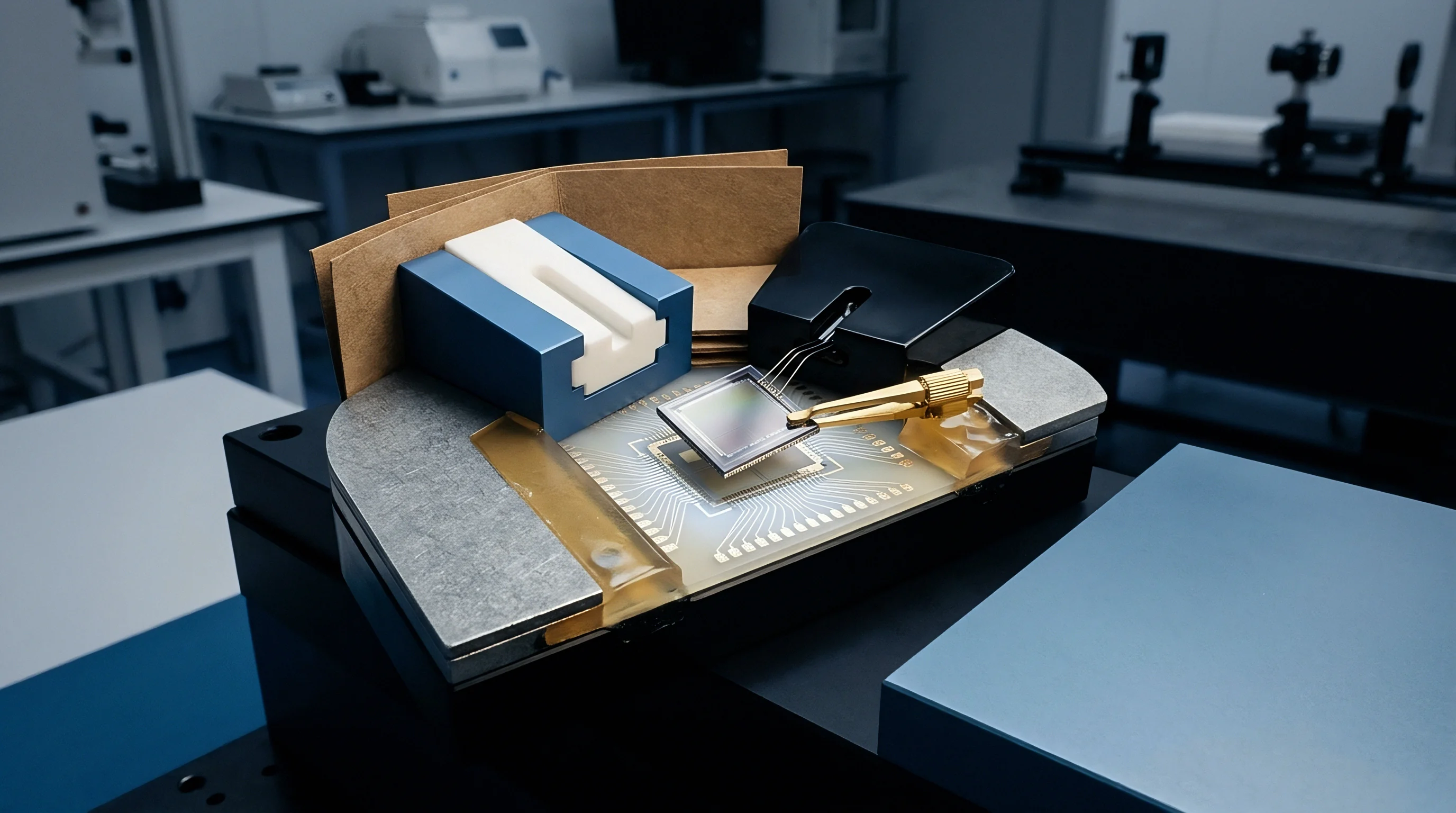
Piezoresistive pressure elements fabricate sensing resistors directly into a micromachined silicon diaphragm using boron ion implantation or thermal diffusion. Single-crystal silicon exhibits a high piezoresistive coefficient, making it sensitive to mechanical strain induced by applied pressure. Temperature changes alter this semiconductor structure through two distinct physical mechanisms operating simultaneously: carrier mobility in p-type silicon decreases as temperature increases due to enhanced lattice phonon scattering, while boron doping density alters these temperature coefficients.
Concurrently, the fundamental piezoresistive shear coefficient degrades at higher thermal energy levels, reducing the output voltage produced per unit of mechanical strain.
The total thermal drift observed at the output terminals splits into Temperature Coefficient of Resistance and Temperature Coefficient of Sensitivity. Doping concentration dictates the magnitudes of both parameters. Lightly doped silicon (1 × 1018 cm-3) yields high pressure sensitivity but suffers from a steep positive resistance coefficient around +0.25%/K and a negative sensitivity coefficient near -0.27%/K. Increasing boron doping density to 1 × 1019 cm-3 stabilizes temperature drift to +0.08%/K and -0.10%/K respectively, though full-scale output drops by more than half.
Designing transducer elements involves selecting a doping profile that trades uncompensated signal output against thermal drift stability.
| Doping Density (cm⁻³) | TCR Range (ppm/K) | TCS Range (ppm/K) | Uncompensated Offset Drift (% FSR/100 K) |
|---|---|---|---|
| 1.0 × 10¹⁸ (P-type) | +1800 to +2500 | -2100 to -2700 | 3.5 to 6.0 |
| 5.0 × 10¹⁸ (P-type) | +1200 to +1600 | -1400 to -1800 | 1.8 to 3.2 |
| 1.0 × 10¹⁹ (P-type) | +600 to +900 | -800 to -1100 | 0.8 to 1.5 |
Zero-pressure offset drift stems from structural asymmetry rather than uniform material shifts. Four piezoresistors arranged in a Wheatstone loop never achieve absolute geometrical or electrical identity. Photolithographic variations of ten nanometers alter absolute resistor values by fractions of a percent, and matching tolerances within 0.05% leave a residual offset that shifts as temperature fluctuates.
Packaging stress further distorts this offset, as differential expansion between the silicon die, borosilicate glass pedestal, and metallic housing imposes mechanical strain directly onto the sensing diaphragm. Glass frit bonding matching pyrex to silicon introduces residual thermal strain across assembly temperatures.
IEC 60770-1 Clause 6.3 mandates continuous temperature stabilization until output drift drops below 0.05 percent FSR per ten-minute window before taking baseline readings.
Thermally induced package stress distorts diaphragm geometry independently of applied fluid pressure. A silicon die with an expansion coefficient of 2.6 × 10⁻⁶/K bonded to a stainless steel header with an expansion coefficient of 16 × 10-6/K experiences bending moments during thermal excursions. Isolating the sensing element using silicone oil fill or compliant organic adhesives dampens mechanical strain transmission at the cost of transient response speed.
Thermal stress relaxation within packaging materials exhibits time-dependent creep, causing baseline calibration shifts over prolonged operating lifespans. Ignoring package-induced strain leads to unrepeatable thermal hysteresis that no downstream electronic calibration can remove.
Soak
Environmental chamber characterization isolates thermal drift parameters from dynamic line transients through controlled thermal cycles. Profiling piezoresistive devices demands mapping bridge output voltage across combined pressure and temperature coordinates. The test system housing the devices must control thermal ramp rates while maintaining pneumatic line stability, since rapid temperature ramps induce internal spatial gradients where the outer metal housing heats faster than the internal silicon element.
Chamber dwell times prevent gradient errors and false hysteresis. Characterization protocols enforce maximum ramp rates of 1.0 °C/min to 1.5 °C/min across the operating temperature range.
Thermal Chamber Dwell Execution
Environmental test profiles enforce multi-point temperature profiles across the sensor operating envelope. Reaching thermal equilibrium at each test temperature plateau requires adequate soak duration: die-level equilibrium requires minimum dwell times of twenty minutes per plateau, whereas oil-filled isolated housings demand forty minutes. Pneumatic pressure generation must remain decoupled from environmental chamber thermal fluctuation.
Pressure lines routed into the chamber require thermal pre-conditioning loops to prevent cold or hot gas injection from biasing die surface readings during measurement sweeps.
- Lower ambient chamber temperature to the lowest specified threshold at a controlled ramp rate of one degree per minute.
- Hold target dwell temperature for thirty minutes to ensure complete internal die equilibrium.
- Step pressure across five calibration points from zero to full scale range using an automated nitrogen pressure generator.
- Record bridge output voltage, excitation current, and integrated internal temperature probe readings simultaneously at each node.
- Repeat pressure sweeps at each thermal dwell step while logging hysteresis between heating and cooling legs.
Thermal equilibrium exists only when internal sensing element temperature tracks chamber air temperature without measurable lead or lag.
Dry nitrogen flushing within the environmental test chamber prevents moisture condensation during transitions below ambient dew points. Water condensation on unsealed sensor pins introduces surface leakage currents that distort microvolt-level Wheatstone bridge measurements. Data acquisition systems logging transducer performance must employ ratiometric voltage sampling to decouple power supply thermal drift from sensor element drift.
High-precision 6.5-digit multimeters or 24-bit delta-sigma converters with temperature-controlled voltage references preserve measurement integrity throughout twenty-four-hour profiling runs. Uncalibrated baseline offset shifts often stem from circuit board assembly soldering stress rather than die attach voiding.
Surface
Bivariate error modeling mapping raw voltage output against pressure and temperature yields the calibration coefficients needed for signal correction. Standard single-variable temperature coefficients assume linear drift profiles, failing to capture high-order silicon piezoresistive behaviors. Real silicon diaphragms demonstrate cross-coupling where the sensitivity drift coefficient varies as a function of applied pressure, and zero-offset drift exhibits non-linear curvature across wide temperature spans.
Constructing a complete surface map requires measuring output voltages across a grid containing at least five temperature points and five pressure points.
Bivariate Polynomial Extraction
Mathematical fits represent pressure sensor transfer functions through multi-variable power series expansions. A second-order bivariate polynomial models output voltage by coupling pressure and temperature terms directly, using matrix inversion and least squares regression to calculate optimal coefficients. The analytical model takes the form:
V_out(P, T) = a_0 + a_1 P + a_2 T + a_3 P T + a_4 T^2 + a_5 P T^2 + a_6 P^2
Evaluating a 100 bar piezoresistive transducer over a -40 °C to +125 °C range demonstrates the efficacy of surface fitting. Uncompensated, the transducer exhibits a span shift of -18.5% FSR and a zero-offset drift of +7.2% FSR. Applying a simple linear offset and span correction reduces residual errors to 1.4% FSR.
Implementing a full second-order bivariate surface model drops total residual thermal error below 0.12% FSR across the entire operating window.
| Model Polynomial Order | Matrix Test Points | Residual TCO Error (% FSR) | Residual TCS Error (% FSR) | EEPROM Storage (Bytes) |
|---|---|---|---|---|
| 1st Order Linear (a₀ + a₁P + a₂T) | 2 Temp × 2 Press | 0.85 | 1.20 | 12 |
| 2nd Order Bivariate (Full Surface) | 3 Temp × 3 Press | 0.08 | 0.12 | 28 |
| 3rd Order Non-Linear Cross-Term | 5 Temp × 5 Press | 0.02 | 0.03 | 56 |
When Does Thermal Hysteresis Overwhelm Digital Trim Correction?
Mechanical packaging mismatch creates non-reversible strain paths during heating and cooling cycles. Thermal hysteresis manifests when a transducer yields differing voltage outputs at 25 °C depending on whether the point was reached from -40 °C or +125 °C. Polynomial algorithms assume a single-valued deterministic output surface for every temperature-pressure pair; when mechanical stress relaxation within elastomeric seals or die-attach adhesives creates non-deterministic output paths, deterministic surface models fail. Strain shifts alter baseline bridge equilibrium, meaning multi-point calibration algorithms cannot correct non-repeatable path-dependent shifts without continuous strain tracking.
A second-order bivariate polynomial fit reduces total uncompensated thermal span drift from 18.5 percent FSR down to 0.12 percent FSR across a 165 Kelvin operating range.
Categorizing thermal drift components ensures correct mathematical compensation modeling.
- Offset Thermal Drift shifts zero-pressure output baseline values as ambient temperature changes across the operating range.
- Span Temperature Drift alters the gain slope, changing millivolt output per unit pressure applied at elevated thermal states.
- Thermal Hysteresis Error causes baseline signal output deviation between ascending and descending thermal sweep directions.
- Non-linear Thermal Coefficient introduces higher-order curvature requiring squared and cubed temperature polynomial variables.
Whether atomic layer deposited thin film coatings can permanently suppress substrate thermal strain accumulation remains open to multi-batch field validation.

Trim
Signal conditioning electronics correct transducer thermal drift using analog element balancing or digital lookup correction. Passive compensation incorporates temperature-stable thin-film resistor networks connected in series or parallel with the piezoresistive bridge. Driving bridges with a constant current source compensates sensitivity loss automatically by exploiting the positive temperature coefficient of resistance as higher temperatures lower piezoresistive shear coefficients.
As temperature rises, total bridge impedance increases, forcing the bridge excitation voltage to rise proportionally and offsetting the sensitivity drop to hold net output span stable within 0.5% FSR over moderate thermal spans.
Excitation Mode Thermal Dynamic Balancing
Driving piezoresistive networks via regulated current sources yields passive baseline temperature compensation. Constant voltage drive lacks this self-compensating mechanism, requiring external gain modification circuits. Active digital compensation replaces passive trim networks by inserting signal conditioning ASICs between the sensing element and host output interface.
Modern conditioning chips integrate a low-noise programmable gain amplifier, a 24-bit analog-to-digital converter, internal temperature sensing diodes, and a digital signal processing engine.

Digital Conditioning ASIC Architecture
Integrated signal processors convert sensor bridge microvolt outputs through high-resolution analog front ends, using internal diodes to provide localized temperature feedback in place of manual laser trimming. The conditioning chip samples bridge output and internal diode temperature simultaneously, applying stored polynomial calibration coefficients in real time. Corrected values drive digital-to-analog converters generating standard 0 to 5 volt signals, 4 to 20 milliamp loops, or digital ratiometric output streams.
Digital ASIC compensation eliminates analog resistor laser trimming steps at the expense of wafer production test cycle time.
Selecting an appropriate thermal drift compensation strategy depends on performance targets and manufacturing capabilities.
- Passive Resistor Trim suits low-cost applications needing simple analog thermal stabilization over narrow operating spans.
- Constant Current Driving provides efficient sensitivity drift cancellation without additional active conditioning microchips.
- Digital ASIC Polynomial Calibration delivers high-accuracy linear output across automotive and aerospace thermal operating envelopes.
Constant current excitation compensates span drift effectively only when resistor temperature coefficients match across all four bridge arms.
Qualification
Production test protocols balance thermal calibration accuracy against manufacturing throughput cost. High-volume sensor manufacturing cannot support extended multi-point temperature matrix calibration for every produced unit due to chamber cycle times. Single-point thermal calibration measures zero-offset drift at room temperature, applying batch-averaged thermal coefficients to correct span drift, though wafer calibration fails under post-assembly thermal stress.
Because multiple thermal steps add significant test expense, high-precision industrial transducers require individual three-point or five-point thermal calibration inside automated environmental indexing chambers.
Production Thermal Calibration Economics
Manufacturing line cycle times depend heavily on the number of thermal soak steps in test routines. Subjecting every sensor module to a full thermal sweep over -40 °C to +125 °C extends production testing time to tens of minutes per device. High-volume automotive applications utilize dual-temperature calibration steps, logging data at room temperature and an elevated temperature point such as +85 °C. This dual-point method corrects baseline offset and linear sensitivity drift while inferring second-order curvature from sample lot qualification data.
| Calibration Strategy | Thermal Soak Points | Test Time per Unit (s) | Residual Thermal Error (% FSR) | Testing Cost Overhead per Unit ($) |
|---|---|---|---|---|
| Batch-Averaged Single Point | 1 (25 °C) | 12 | 1.80 to 3.50 | 0.15 |
| Dual Point Individual Trim | 2 (25 °C, 85 °C) | 240 | 0.35 to 0.70 | 1.25 |
| Full Matrix Bivariate Surface | 5 (-40 °C to 125 °C) | 1800 | 0.05 to 0.15 | 6.50 |
| Testing overhead estimates reflect multi-socket chamber operational costs and nitrogen consumption per unit. | ||||
Transducer qualification standards define rigorous thermal stress testing sequences to guarantee long-term stability. Standard AEC-Q103-002 specifies qualification requirements for MEMS pressure sensors in automotive applications, including thermal shock exposure from -40 °C to +150 °C for 1000 cycles. Transducers undergoing qualification testing must demonstrate post-test thermal offset shift below specified limits.
Thermal cycling accelerates mechanical stress relaxation in packaging materials, exposing micro-cracks in die attach glass frits and wire bond bonds. AEC-Q103-002 Clause 4.2 mandates post-reflow thermal drift re-characterization, which invalidates wafer-level calibration data if board assembly stress alters die zero-offset.