Modeling Hydrostatic Pressure Effects on Transducer Hysteresis and Long Term Drift Limits
Hydrostatic pressure drives viscoelastic oil relaxation and silicon lattice creep, turning unmodeled transducer hysteresis into major long-term zero drift.

Diaphragm
Isolation Seals and Fluid Compression Physics
Pressure measurement at high hydrostatic levels relies on mechanical isolation assemblies that transmit fluid force while shielding internal sensing elements from corrosive media. Oil-filled piezoresistive cells utilize a thin, convoluted metallic membrane to separate seawater or hydraulic fluid from a silicone oil cavity. The bulk modulus of the oil cavity dictates the volumetric deflection under hydrostatic loading.
As ambient hydrostatic pressure increases to 70 MPa, the oil volume compresses by roughly 3.5 percent. Pressure distorts metal. This compression forces the isolating element inward, introducing mechanical bending stresses independent of the applied differential pressure line.
Viscoelastic relaxation in synthetic fill fluids creates a time-dependent pressure distribution against the internal transducer capsule. Silicone oils exhibit shear-rate independence at ambient conditions, yet under continuous hydrostatic pressures exceeding 40 MPa, molecular compaction increases dynamic viscosity. This viscous resistance delays pressure equalization across internal passages during rapid pressure steps, manifesting as transient zero offsets.
The mechanical interface between the outer metallic housing, glass-to-metal header seals, and the internal silicon element forms a complex stress loop. Each material in this chain possesses a distinct bulk modulus and thermal expansion coefficient, generating localized shear stresses under deep-water submersion.
Synthetic fluid compression introduces non-linear structural deflection along the sensing membrane before active pressure strain reaches the transducer bridge.

Mechanical Strain Transmission across Wetted Interfaces
Force transmission from the fluid medium to the strain-sensitive element is governed by the structural compliance of the wetted assembly. In high-pressure applications, the edge constraints of the isolating membrane experience high localized bending moments. Metallic membranes subjected to repeated hydrostatic cycles exhibit work-hardening at these circumferential flexure points.
Work-hardening alters the spring rate of the membrane, shifting the transducer sensitivity constant over extended service periods.
Isolation designs incorporating elastomeric O-rings present additional hysteresis mechanisms. Elastomers under 50 MPa hydrostatic pressure experience micro-extrusion into sealing gaps, alongside volumetric compression. When hydrostatic line pressure decreases, the constrained elastomer releases stored elastic energy at a rate governed by its internal friction coefficient.
This delayed mechanical recovery exerts a residual clamping force on the sensor body, distorting the bridge baseline calibration. The sensor manufacturer attributes the zero offset shift after deep ocean submersion to standard seal bedding rather than structural lattice displacement.
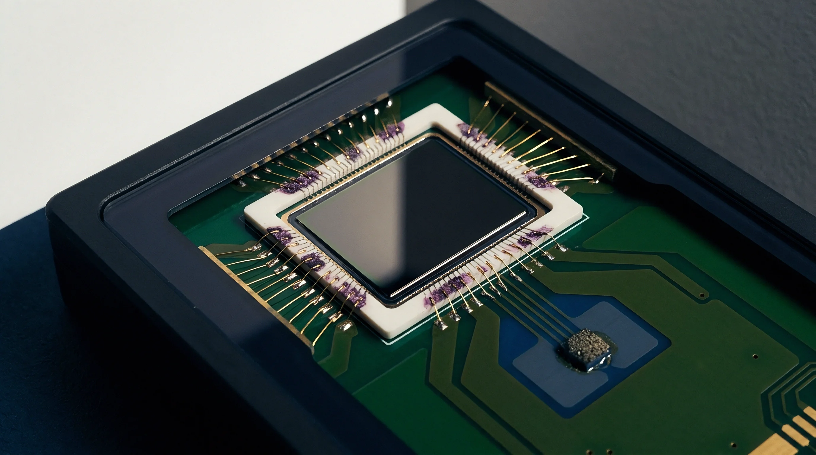

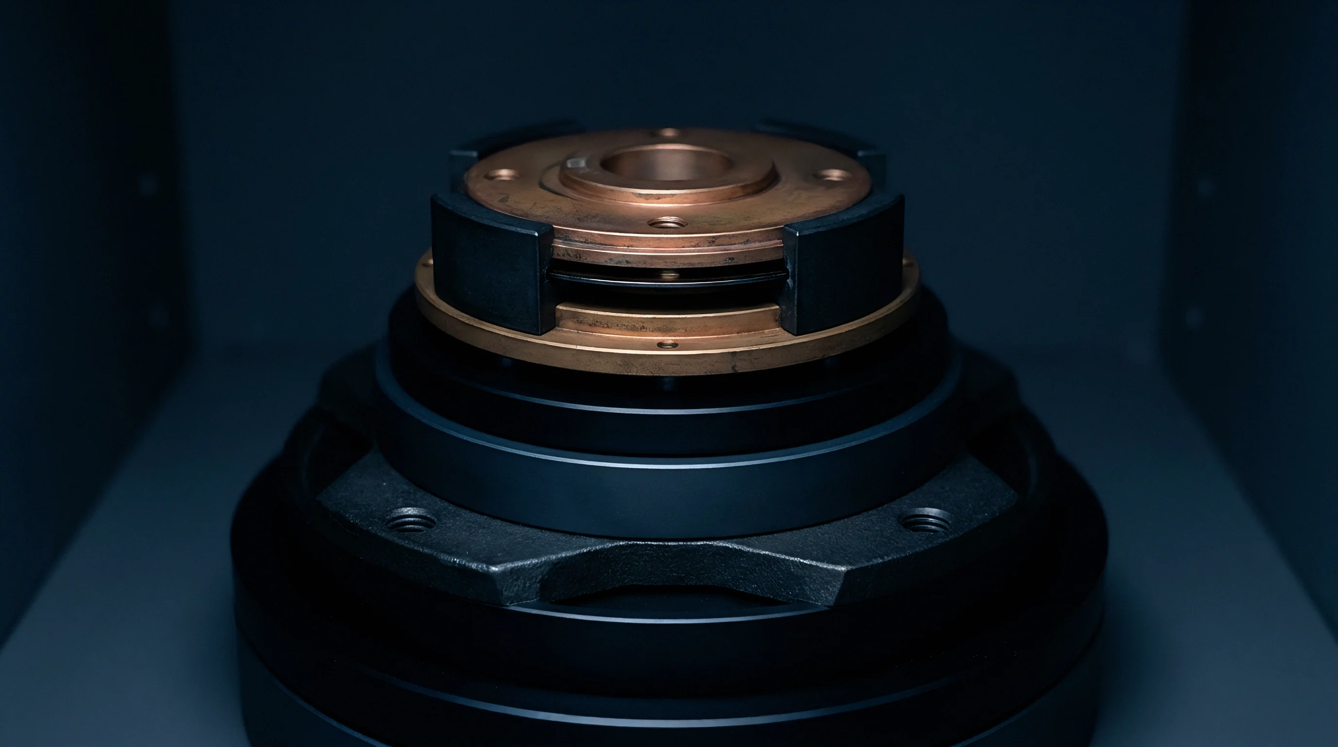
Lattice

Micro-Yielding and Dislocation Kinetics in Monocrystalline Silicon
Monocrystalline silicon serves as the piezoresistive transducer element due to its near-perfect elastic behavior at moderate strain levels. Under high hydrostatic stress, micro-scale defects within the silicon crystal structure govern non-linear mechanical responses. Lattice slip alters zero.
Imperfections such as vacancies, interstitial atoms, and edge dislocations act as localized stress concentrators when subjected to triaxial hydrostatic compression.
Continuous exposure to hydrostatic pressures above 50 MPa lowers the activation energy required for dislocation movement along the prime slip planes of silicon. Micro-yielding occurs when localized shear stress exceeds the theoretical yield strength of the crystal locally, even while the macro-structure remains well within its nominal elastic limit. Stresses remain active.
This micro-yield mechanism produces irreversible atomic realignments. Upon pressure release, the silicon substrate fails to return to its initial spatial geometry, leaving a residual strain field across the diffused piezoresistors.
| Transducer Core Type | Dominant Hysteresis Mechanism | Typical 1-Year Zero Drift (70 MPa Load) | Viscoelastic Relaxation Time | Recovery Period Post-Depressurization |
|---|---|---|---|---|
| Silicon Piezoresistive (Oil-Filled) | Oil compression and header shear strain | 0.12% Full Scale | 48 to 72 Hours | 120 Hours |
| Thin-Film Strain Gauge (Sputtered) | Substrate micro-yield and grain boundary slip | 0.05% Full Scale | 12 to 24 Hours | 36 Hours |
| Ceramic Capacitive (Alumina) | Joint adhesive creep and hysteresis in seals | 0.08% Full Scale | 36 to 90 Hours | 96 Hours |
| Quartz Crystal Resonator | Crystal resonator mount elastic relaxation | 0.01% Full Scale | 2 to 6 Hours | 12 Hours |
Stress-Induced Anelastic Strain and Hysteresis Loop Formation
Anelasticity describes the time-dependent, reversible strain component that lags behind applied hydrostatic stress. Unlike plastic deformation, anelastic strain fully recovers over extended dwell periods at zero pressure. Sensor hysteresis manifests as the path difference between ascending and descending calibration curves, directly driven by this anelastic retardation.
During pressure ramp-up, energy is stored within point defect clusters; during pressure ramp-down, internal friction prevents immediate energy release.
The width of the hysteresis loop correlates directly with peak hydrostatic exposure pressure and dwell duration at maximum load. Long dwell times allow maximum anelastic strain saturation, maximizing the zero-offset error upon immediate return to atmospheric pressure. Creep alters span.
The physical mechanisms contributing to structural relaxation and degradation under hydrostatic loading fall into distinct physical categories:
- Lattice Defect Migration movement of point vacancies within the single-crystal matrix under directional shear stresses.
- Bond Line Relaxation mechanical stress decay within glass-frit and epoxy die-attach layers joining the sensor chip to its header.
- Fill-Fluid Gas Absorption dissolved gas phase changes within the isolation oil under high-pressure hydrostatic compression.
- Housing Material Creep localized yielding of 316L stainless steel or Inconel sensor bodies surrounding the sensing capsule.
Ignoring micro-yield deformation in deep-water pressure cells yields systematic calibration errors exceeding ten times the baseline instrument uncertainty over three service years.

Formulation
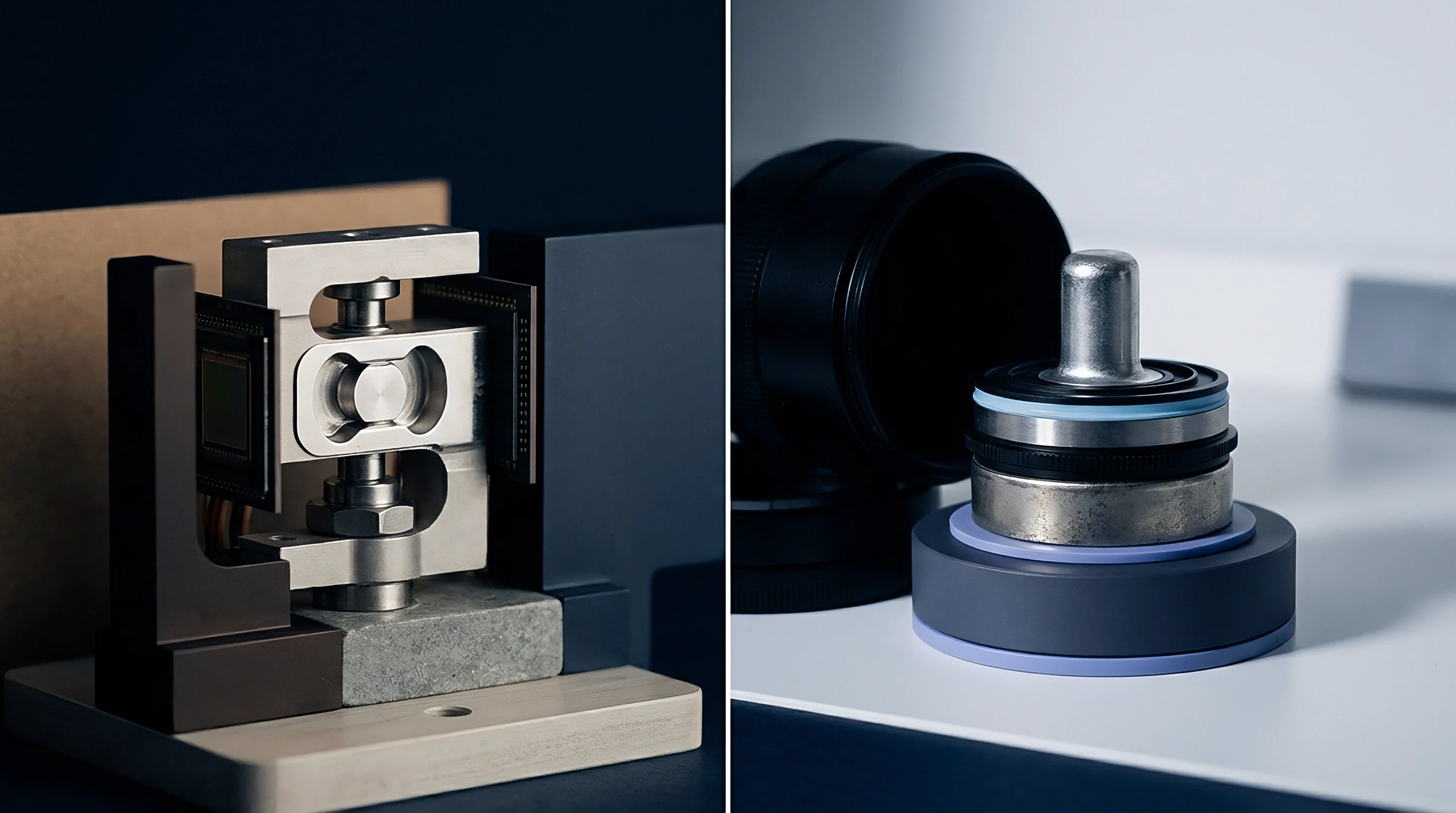
Mathematical Construction of Hydrostatic Hysteresis
Modeling hydrostatic pressure effects demands decoupled formulations for instantaneous elastic deformation, history-dependent hysteresis, and long-term time-dependent drift. Total sensor output voltage is represented as a linear combination of these distinct physical components. The mathematical representation of the pressure-dependent hysteresis voltage relies on a modified Duhem operator, mapping output path variations relative to the directional derivative of applied pressure.
The immediate elastic response follows a second-order polynomial accounting for non-linear pressure-strain conversion. The dynamic hysteresis component relies on an integral form containing an exponential memory kernel. This kernel weighs past pressure states, decaying as a function of pressure history interval.
Sensors drift slowly. Data proves strain. The mathematical continuous formulation takes the form:
V(P, t) = V_zero + S_0 P (1 + C_np P) + H_p(P, dP/dt) + D_t(P, t)
Here, V_zero represents the baseline zero-pressure output, S_0 is the primary sensitivity factor, C_np is the non-linearity coefficient, H_p is the path-dependent hysteresis function, and D_t is the time-dependent drift accumulation. The term H_p is modeled as:
H_p(P, dP/dt) = gamma integral d-tau
The parameter gamma scales hysteresis amplitude based on peak line pressure, while alpha dictates the memory decay rate of structural anelasticity within the assembly materials.

Time-Dependent Creep and Zero Drift Equations
Long-term drift under constant hydrostatic pressure follows logarithmic time-dependency, characteristic of primary creep in solid-state crystalline materials and polymeric seals. The cumulative zero-point drift equation expresses baseline wander as a function of continuous pressure exposure duration and ambient operating temperature:
D_t(P, t) = A_drift (P / P_ref)^beta ln(1 + t / t_0) exp(-E_a / (k T))
In this equation, A_drift represents the empirical material drift scaling coefficient, P_ref is the reference calibration pressure, beta is the pressure-stress acceleration exponent, t_0 is the relaxation time constant, E_a is the thermal activation energy of the dominant creep mode, k is the Boltzmann constant, and T is absolute temperature in Kelvin.
When Does Oil-Fill Viscoelastic Relaxation Dominate Silicon Diaphragm Micro-Creep?
Internal fluid compression and molecular ordering processes dominate the total sensor drift signature during the initial 72 hours of constant pressure exposure. Beyond 100 hours of continuous submersion, the rate of viscoelastic strain decay in synthetic oil drops below the continuous creep rate of the crystal lattice and mechanical die-attach joints. Oil compresses under load.
Structural creep in metal-to-silicon mounting interfaces becomes the primary driver of zero-point drift over multi-year deployments.
To demonstrate this formulation, assume a subsea transducer operates under a constant hydrostatic pressure of 70 MPa at 277 Kelvin. The baseline parameters are specified as A_drift = 0.05 percent Full Scale, beta = 1.35, P_ref = 50 MPa, t_0 = 1 hour, and E_a = 0.35 electron-volts. Over an operational period of 8,760 hours (one calendar year), the continuous pressure stress factor yields a multiplier of 1.57 relative to baseline.
The logarithmic time factor across 8,760 hours computes to ln(8761) = 9.078. Combining these factors with the thermal attenuation term yields a predicted zero-point drift limit of 0.28 percent of Full Scale for the first year. If peak hydrostatic exposure increases to 100 MPa, the predicted zero drift shifts to 0.45 percent Full Scale due to the non-linear exponent beta.
Hysteresis scales quadratically with peak exposure pressure, whereas long-term zero drift scales logarithmically with continuous immersion time.

Rig
Primary Pressure Reference Standards and Deadweight Testers
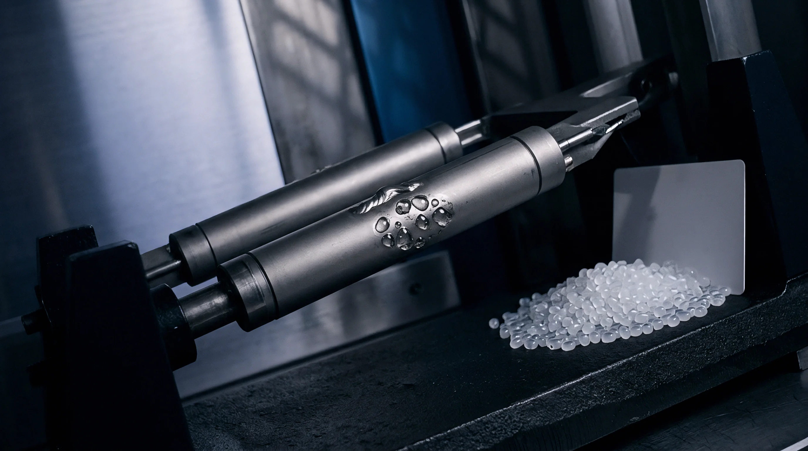
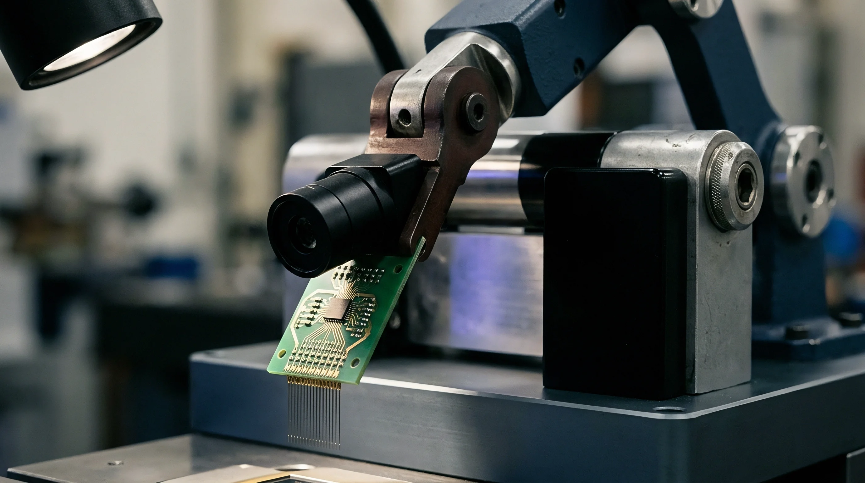
Quantifying transducer hysteresis and long-term drift limits demands a hydraulic calibration apparatus capable of generating precise pressure steps while isolating thermal artifacts. Automated primary deadweight testers utilizing tungsten carbide piston-cylinder assemblies serve as the baseline pressure reference. These systems achieve measurement uncertainties under 0.005 percent of reading by compensating for local gravitational acceleration, air buoyancy on floating masses, and thermal expansion of the piston-cylinder area.
The fluid medium within the test loop must match the operational compatibility of the device under test. Hydraulic oil calibration loops require precise temperature stabilization within a fluid bath controlled to within 0.01 degrees Celsius. Thermal fluctuations introduce pressure variations via fluid expansion inside clamped test lines, confounding true mechanical hysteresis measurements with thermally induced zero shifts.
The primary pressure reference standard must maintain an uncertainty budget three times tighter than the combined hysteresis and drift tolerance of the sensor under test.
Sequential Cycling Protocols for Hysteresis Isolation
Characterizing pressure hysteresis requires a strictly controlled, multi-step pressure sequence to separate instantaneous elastic response from time-dependent creep. Seals deform slowly. The incoming inspection protocol uses a baseline calibration routine to quantify performance metrics:
- Thermal Stabilization Hold the device under test at ambient calibration temperature within the fluid bath for four hours at zero pressure to eliminate thermal gradients.
- Pre-Conditioning Cycles Exercise the transducer through three full-scale pressure cycles from atmospheric pressure to maximum rated line pressure, holding at peak for two minutes per cycle to work-harden mechanical joints.
- Ascending Step Calibration Apply hydrostatic pressure in ten equal increments from zero to 100 percent of full scale, holding each step for exactly 60 seconds before recording output voltage.
- Peak Pressure Dwell Maintain maximum test pressure for 24 hours to saturate short-term anelastic strain and short-term fluid viscoelastic relaxation modes.
- Descending Step Calibration Decrease pressure through the identical ten step increments, recording output voltage at each 60-second mark to capture the descending response path.
- Zero-Point Recovery Tracking Vent system pressure to atmosphere and record the zero-offset voltage continuously at 1-minute intervals for 48 hours to chart the anelastic recovery curve.
ISO/IEC 17025 Clause 7.8.4 requires explicitly stating the coverage factor and pressure history on calibration certificates, turning ambiguous manufacturer stability claims into auditable bounds.

Uncertainty
Budgeting Hydrostatic Drift in Subsea Measurement Chains
Constructing a metrologically sound uncertainty budget for high-pressure transducers requires combining independent error sources according to the Guide to the Expression of Uncertainty in Measurement. Standard accuracy statements on vendor datasheets typically include only terminal non-linearity, baseline thermal error, and ambient bench hysteresis. They regularly omit long-term creep and hydrostatic line-pressure sensitivity coefficients.
Line pressure effects alter both the offset and the effective span of the sensor. Uncertainty grows with time. When calculating expanded uncertainty for subsea monitoring installations, engineers root-sum-square the standard uncertainties of individual terms after scaling by their sensitivity coefficients.
Errors compound quickly. The combined standard uncertainty u_c integrates thermal, mechanical, and pressure-induced instabilities into a unified metric.
| Uncertainty Component Source | Standard Uncertainty (u_i) | Probability Distribution Type | Sensitivity Coefficient (c_i) | Uncertainty Contribution (% FS) |
|---|---|---|---|---|
| Primary Reference Calibration Standard | 0.0025% FS | Normal (k = 2) | 1.0 | 0.0025% |
| Pressure-Induced Zero Hysteresis | 0.0450% FS | Rectangular | 1.0 | 0.0260% |
| Time-Dependent Creep (36 Months) | 0.1600% FS | Rectangular | 1.0 | 0.0924% |
| Fluid Viscoelastic Memory Effect | 0.0300% FS | Triangular | 1.0 | 0.0122% |
| Thermal Coefficient Drift (5 deg C delta) | 0.0200% FS | Normal (k = 1) | 1.0 | 0.0200% |
| Power Supply Regulation Variation | 0.0050% FS | Rectangular | 1.0 | 0.0029% |
Expanded Measurement Uncertainty and Coverage Factors
To convert combined standard uncertainty into expanded uncertainty, the laboratory applies a coverage factor k based on the degrees of freedom determined via the Welch-Satterthwaite equation. For measurement chains with high effective degrees of freedom, a coverage factor of k = 2 establishes a confidence level of approximately 95 percent.
Calculating the total expanded uncertainty from the budget table values proceeds by summing the squared contributions. Combining 0.0025 squared, 0.0260 squared, 0.0924 squared, 0.0122 squared, 0.0200 squared, and 0.0029 squared yields a total variance of 0.00977. Taking the square root gives a combined standard uncertainty u_c of 0.0988 percent Full Scale.
Multiplying by a coverage factor of k = 2 produces an expanded uncertainty of 0.1976 percent Full Scale. Long-term continuous hydrostatic creep dominates this total budget, representing over 85 percent of the variance pool.
Verification documentation must explicitly itemize key operating conditions to satisfy quality standards:
- Hydrostatic Pressure History complete record of peak pressure exposures, dwell times, and ramp rates prior to calibration testing.
- Thermal Exposure Bounds environmental temperature limits maintained throughout the measurement and calibration sequence.
- Traceable Reference Certificates unique identification codes linking primary deadweight standards to national metrology institutes.
- Coverage Factor Justification mathematical derivation of the effective degrees of freedom and corresponding confidence interval selections.
The precise threshold where cyclic dislocation movement transitions into permanent crystal lattice slip remains unquantified across commercial MEMS pressure cells operating above one hundred megapascals.


Expenditure

Commercial Mechanics of Tight Hysteresis Specifications
Procuring pressure transducers with tightly bounded hysteresis limits shifts substantial financial expenditure onto incoming test procedures and vendor yield management. Sensor manufacturers price high-accuracy grades based on calibration sorting yields rather than fundamental differences in raw materials or structural assembly. Bonds relax under stress.
A pressure transducer specified for 0.05 percent Full Scale hysteresis requires extended burn-in cycles and multi-point pressure screening at elevated temperatures. Pressure shifts the baseline. Standard commercial units with 0.25 percent Full Scale hysteresis limits undergo simple two-point room-temperature trimming, minimizing factory bench time.
Specifying an accuracy class one step tighter than operational requirements reduces qualified vendor counts and increases unit acquisition costs exponentially.
Purchasing unverified low-drift sensor models creates downstream financial liability when unbudgeted field re-calibrations become necessary to prevent process downtime.
Re-Calibration Interval Economics and Field Recalls
Long-term hydrostatic zero drift directly dictates the preventive maintenance and re-calibration schedule for deep-sea installations and high-pressure industrial process plants. Subsea retrieval of pressure monitoring hardware incurs offshore vessel charter costs ranging from 50,000 to 150,000 USD per day. Selecting a sensor based solely on initial purchase price without accounting for hydrostatic creep rates leads to premature re-calibration intervals.
Take an offshore installation utilizing 20 subsea pressure transmitters. Selecting Grade A transducers with verified drift limits of 0.03 percent Full Scale per year allows a 5-year field service interval. Grade B transducers with unverified drift limits of 0.15 percent Full Scale per year force a 2-year re-calibration cycle to maintain process safety margins.
Over a 10-year platform lifecycle, Grade B hardware demands three additional offshore retrieval campaigns, costing millions of dollars in field intervention expense. Upfront investment in verified low-creep sensor designs reduces overall life-cycle expenditure, demonstrating that low initial component cost often represents the most expensive long-term engineering choice.