Discrete Kalman Process Noise Covariance Derivation from Inertial Bench Test Metrics
Bench Allan variance parameters convert to discrete Kalman process noise matrices by integrating state transition matrices over the sampling interval.
Trace
Static bench measurements of inertial sensors establish the baseline stochastic profile needed to populate continuous state-space noise matrices. Translating raw sensor output into a mathematical error model requires isolating individual noise mechanisms operating across distinct time scales. Micro-electro-mechanical systems (MEMS) accelerometers and gyroscopes display stochastic behaviors dominated by white noise at high frequencies, flicker noise at mid-band frequencies, and random walk dynamics over extended periods.
Characterizing these noise components relies on long-duration static data collection in a thermally stable environment isolated from external structural vibrations.
Allan variance analysis serves as the primary analytical tool for decomposing stationary time-series data into specific noise coefficients, following procedures codified in IEEE Std 952 for gyroscopes and IEEE Std 1431 for accelerometers. A continuous data record captured at a constant sampling frequency is divided into cluster lengths of duration tau. Calculating the sample mean of each cluster and taking the expected value of the squared differences between consecutive cluster means generates the Allan variance curve as a function of cluster duration.
Plotting the square root of the Allan variance, known as the Allan deviation, on a log-log scale surfaces distinct gradient slopes corresponding to specific physical noise phenomena.
The log-log Allan deviation plot exhibits five primary region slopes, each directly mapping to a specific stochastic process. A slope of negative one-half indicates white noise, quantified as Angle Random Walk (ARW) for rate gyroscopes in units of degrees per square root hour, or Velocity Random Walk (VRW) for accelerometers in units of meters per second per square root hour. The flat region with a slope of zero identifies the in-run bias instability, representing the minimum achievable bias uncertainty under constant temperature.
Positive slopes of plus one-half reflect Rate Random Walk (RRW) or Acceleration Random Walk (AccRW), which describe long-term sensor bias drift driven by environmental fluctuations and internal physical aging.
| Noise Process Type | Allan Variance Slope | Allan Deviation Notation | Sensor Metric Units | State Noise Coefficient Symbol |
|---|---|---|---|---|
| Quantization Noise | -1.0 | Q | rad or m/s | S_q |
| Angle / Velocity Random Walk | -0.5 | N (ARW / VRW) | rad/s^0.5 or m/s^1.5 | q_w |
| In-Run Bias Instability | 0.0 | B | rad/s or m/s^2 | q_b |
| Rate / Acceleration Random Walk | +0.5 | K (RRW / AccRW) | rad/s^1.5 or m/s^2.5 | q_k |
| Ramp Noise / Drift Rate | +1.0 | R | rad/s^2 or m/s^3 | q_dr |
Extracting the continuous noise power spectral density matrix from these Allan deviation plots demands exact unit conversion. Datasheets frequently state white noise as a spectral density figure, such as micro-g per square root Hertz for accelerometers or degrees per hour per square root Hertz for gyroscopes. Converting Angle Random Walk from degrees per square root hour to continuous rate white noise spectral density q_w in radians squared per second requires dividing by sixty and applying the degree-to-radian transformation.
Static bench testing of a MEMS rate gyroscope at 25 degrees Celsius yields an angle random walk of 0.08 degrees per square root hour when sampled at 1000 Hz over a twelve-hour window.
Continuous process noise models rely on precise mathematical mapping from time-domain variance metrics to frequency-domain power spectral densities. For Angle Random Walk N, the equivalent continuous white noise power spectral density q_w equals N squared when N expressed in SI units of radians per root second. For Rate Random Walk K, the continuous driving white noise density q_k entering the derivative of the bias state equals three times K squared when K expressed in radians per second to the three-halves power.
Establishing these numerical values from static test data completes the identification phase, providing the raw inputs needed to form the continuous process noise matrix.
- Data Collection Sequence ~ Mount the inertial sensor on an isolated optical table inside a temperature-controlled chamber maintained within 0.1 degrees Celsius, logging stationary sensor outputs at full digital bandwidth for sixteen consecutive hours.
- Data Preprocessing Step ~ Remove initial thermal transients by trimming the first thirty minutes of data, and inspect the time series for uncompensated physical shock spikes or communication frame drops.
- Allan Variance Computation ~ Compute the sample variance of consecutive cluster means across integration durations ranging from the inverse sampling rate up to one-third of the total dataset duration.
- Logarithmic Curve Fitting ~ Identify the negative one-half slope region at tau equals one second to extract Angle Random Walk, and pinpoint the zero-slope minima to extract the in-run bias stability coefficient.
- Spectral Density Conversion ~ Convert extracted Allan deviation coefficients into continuous-time power spectral density values formatted in standard metric units for direct insertion into continuous covariance matrices.
Omitting rate random walk slopes during long-duration stationary bench testing leads to an unmodeled bias covariance expansion that degrades state estimations within three hours of continuous operation.
Discretization
Translating continuous-time power spectral densities into discrete state covariance elements requires integrating the state transition dynamics over the sampling step. Linear state-space systems model the evolution of error states using a continuous differential equation driven by continuous white noise. The Kalman filter operates on digital computing hardware, executing state updates at discrete temporal increments designated by dynamic interval delta_t.
Calculating the discrete process noise covariance matrix Q_k involves solving a matrix integral that blends continuous state dynamics with continuous noise intensity values across each discrete sampling step.
The exact analytical expression for the discrete process noise covariance matrix Q_k depends on the state transition matrix Phi and the continuous process noise distribution matrix G. Mathematically, Q_k equals the integral from zero to delta_t of Phi of tau, multiplied by G, multiplied by continuous power spectral density matrix Q_c, multiplied by G transpose, multiplied by Phi transpose of tau, integrated over variable tau. When the continuous system matrix F remains time-invariant across integration duration delta_t, the state transition matrix Phi of tau simplifies to the matrix exponential of F times tau.

Matrix Exponential Integration Techniques
Numerical evaluation of the continuous covariance integral presents challenges when state matrices contain non-zero off-diagonal coupling terms. Direct numerical integration via Simpson rule or trapezoidal quadrature introduces approximation errors when sampling frequency approaches system bandwidth limits. The Van Loan method provides an exact, computationally stable algorithm for computing both the discrete state transition matrix Phi_k and discrete process noise covariance Q_k simultaneously using a single matrix exponential computation.
Constructing the Van Loan block matrix demands forming a 2n-by-2n matrix divided into four n-by-n sub-blocks. Matrix A occupying the upper-left block equals negative F. Matrix B occupying the upper-right block equals G multiplied by Q_c, multiplied by G transpose. Matrix C in the lower-left block equals an n-by-n zero matrix, while matrix D in the lower-right block equals F transpose.
Computing the matrix exponential of this 2n-by-2n matrix multiplied by step duration delta_t yields a structured block matrix result. The upper-right block of this exponentiated result, multiplied by the transpose of the lower-right block, generates the exact discrete process noise covariance matrix Q_k without numerical integration loss.
Compliance with IEEE Std 952 Annex C requires temperature stabilization to within 0.1 degrees Celsius during static data collection to prevent thermal drift from obscuring rate random walk slopes.
Simplified low-order polynomial expansions offer alternative discretization routes when processing power restricts matrix exponentiation. Expanding the state transition matrix Phi of tau as an identity matrix plus F times tau reduces the continuous integral to a truncated power series. For zero-order approximations where F tau terms are neglected, discrete covariance Q_k simplifies to G times Q_c, multiplied by G transpose, multiplied by step length delta_t.
For second-order approximations, additional cross-coupling terms proportional to delta_t squared and delta_t cubed emerge, capturing kinematic velocity-to-position covariance growth within the discrete step.
Truncating the matrix exponential expansion after the first term creates artificial filter instability whenever state transition dynamics move faster than the measurement update interval.

Derivation
Calculating the discrete process noise covariance matrix for a 6-DoF error state starts with the physical continuous spectral density values obtained from static bench testing. Consider a standard inertial error model incorporating three position errors, three velocity errors, three attitude errors, three accelerometer bias errors, and three gyroscope bias errors. Defining the attitude and bias dynamics allows building a fully coupled twelve-state continuous linear model.
The continuous state noise matrix Q_c contains diagonal sub-matrices corresponding to accelerometer velocity random walk, gyroscope angle random walk, accelerometer bias rate random walk, and gyroscope rate random walk.
Formulating the continuous system matrix F establishes the kinematic couplings between states. Position derivative maps directly to velocity. Velocity derivative couples to attitude errors through gravity vector orientation and specific force measurements.
Bias derivative states connect directly to driving continuous white noise sources. Constructing continuous matrix G maps driving noise inputs directly to their corresponding state derivatives. Gyroscope rate white noise enters attitude error derivatives, while accelerometer acceleration white noise enters velocity error derivatives.
Bias instability drift terms enter the derivatives of the respective sensor bias states.

Does Sampling Frequency Alter Continuous Noise Power Conversion?
Higher data update rates compress the integration interval while scaling discrete process noise covariance proportionally to step duration. Assume a tactical-grade MEMS IMU operating at a discretization rate of 200 Hz, corresponding to step length delta_t equal to 0.005 seconds. Bench metrics extracted from Allan variance reveal an Angle Random Walk of 0.1 degrees per square root hour, translating to continuous gyro white noise density q_w equal to 8.461 times 10 to the power of negative 10 radians squared per second cubed.
Velocity Random Walk measures 50 micro-g per square root Hertz, yielding continuous accel noise density q_v equal to 2.406 times 10 to the power of negative 7 meters squared per second cubed. Gyro bias instability yields a rate random walk coefficient q_bg equal to 1.50 times 10 to the power of negative 14 radians squared per second to the fifth power.
Integration interval duration dictates discrete covariance magnitude. Evaluating the discrete covariance terms for a single axis of velocity v and position p under continuous white acceleration noise q_v demonstrates the mathematical derivation of off-diagonal coupling terms. Integrating the state transition matrix over step length delta_t yields specific discrete variance and covariance values for position and velocity errors.
Position error variance due to acceleration noise equals one-third times q_v, multiplied by delta_t cubed. For delta_t equal to 0.005 seconds, this term equals 1.0025 times 10 to the power of negative 14 meters squared. Velocity error variance due to acceleration noise equals q_v multiplied by delta_t, yielding 1.203 times 10 to the power of negative 9 meters squared per second squared.
Cross-covariance between position error and velocity error equals one-half times q_v, multiplied by delta_t squared, yielding 3.0075 times 10 to the power of negative 11 meter-seconds. Constructing discrete matrix Q_k using these explicit algebraic terms preserves physical cross-correlations generated by system kinematics across each sample interval.
| Integration Method | Mathematical Expression for Q_k | Off-Diagonal Term (Pos-Vel) | Computation Cycle Time | Discretization Error Magnitude |
|---|---|---|---|---|
| Zero-Order Euler Approximation | G Q_c G^T delta_t | 0.000 | 0.2 micro-sec | High (Truncation Error) |
| First-Order Kinematic Expansion | Integral of (I + F tau) G Q_c G^T (I + F tau)^T | 0.5 q_v delta_t^2 | 1.2 micro-sec | Low (Exact for Const Acc) |
| Van Loan Matrix Exponential | Upper-Right Submatrix Product via Exponentiation | 0.5 q_v delta_t^2 + O(delta_t^3) | 8.5 micro-sec | Zero (Machine Precision) |
Attitude error variance derived from gyro white noise q_w scales linearly with step length. Discrete attitude variance per axis equals q_w multiplied by delta_t, yielding 4.2305 times 10 to the power of negative 12 radians squared at 200 Hz. In-run bias variance terms scale with step duration, adding small diagonal elements equal to q_bg multiplied by delta_t to the discrete bias covariance blocks. Filter stability hinges on accurate covariance bounds.
Process noise covariance matrices built purely from static bench tests underestimate real position error propagation whenever mechanical vibration excites sensor resonant modes.
Whether off-diagonal cross-axis noise terms can be safely set to zero in high-g maneuver environments remains an open trade-off between processor clock cycles and positioning accuracy.

Discrepancy
Static bench test metrics fail to capture the additional stochastic power generated under operational dynamics. Ambient thermal gradients, structural flexure, power rail ripple, and high-frequency acoustic noise shift effective sensor noise levels far above baseline laboratory measurements. Linear accelerometers tested on an isolated granite block exhibit exceptionally low white noise figures, yet demonstrate significant output corruption when subjected to wideband mechanical vibration.
This phenomenon requires applying dynamic tuning multipliers to bench-derived process noise matrices prior to deploying filters in operational environments.
Bench Noise versus Dynamic Field Shift
Vibration rectification alters the effective zero-rate offset of MEMS comb structures when subject to broadband linear acceleration. Asymmetric mechanical stops and non-linear spring constants inside the silicon die convert high-frequency oscillatory motion into steady-state DC offset shifts. This mechanical rectification cannot be modeled as pure additive white noise.
System integrators accommodate vibration rectification by artificially scaling continuous velocity random walk parameters q_v by factors ranging from two to ten based on empirical field data. High bandwidth reduces sample phase delay.
Rapid environmental temperature changes generate non-uniform thermal expansion across the ceramic package, inducing mechanical stress on the suspended MEMS proof mass. This stress manifests as a transient bias drift that overwhelms standard in-run bias stability metrics captured under isothermal bench conditions. Thermal rate of change, expressed in degrees Celsius per minute, correlates directly with additional rate random walk magnitude.
Process noise covariance matrices must expand their bias random walk diagonal terms when operating across dynamic thermal profiles.
- Vibration Rectification Error ~ Non-linear mechanical rectification converts high-frequency structural shaking into low-frequency sensor bias shifts, elevating effective velocity random walk values.
- Cross-Axis Sensitivity Coupling ~ Structural orthogonality errors between internal sensor axes leak high-amplitude motion energy into orthogonal measurement channels during multi-axis maneuvers.
- Package Thermal Stress Transients ~ Temperature change rates induce internal mechanical strain gradients across silicon flexures, driving transient bias shifts that exceed static Allan variance bounds.
- Power Supply Ripple Injection ~ Voltage regulator noise and digital switching transients leak through sensor analog circuitry, increasing white noise density at specific operational clock harmonics.
- Quantization Noise Foldback ~ High-frequency mechanical vibrations exceeding half the sensor sampling frequency alias into the digital passband, raising the low-frequency noise floor.
Axis misalignment adds correlated process cross-talk. Manufacturing tolerances limit internal die alignment to within 0.1 degrees of package walls. Cross-axis sensitivity causes linear acceleration along one axis to generate spurious readings on orthogonal axes.
In dynamic environments involving high linear acceleration, cross-axis coupling injects correlated noise across independent filter states. Populating off-diagonal terms in continuous noise matrix Q_c models this cross-axis energy transfer, preventing state estimation covariance from collapsing to overly optimistic confidence bounds.
Digitization noise dominates the short-term Allan variance plot when sensor quantization step size exceeds the internal analog noise floor.
Suppliers frequently attribute unexpected field drift to uncompensated structural strain on the printed circuit assembly rather than internal die-level stress.
Ledger
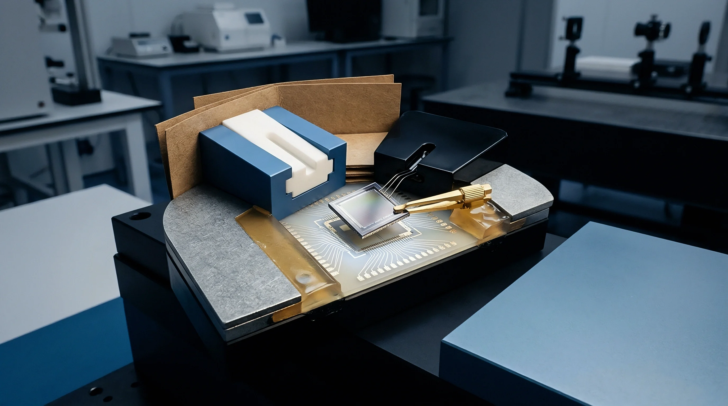
Sensor selection determines both hardware unit cost and the long-term engineering effort needed to maintain filter convergence in production. Sourcing inertial measurement units involves balancing physical performance metrics against landed component costs, supply chain stability, and qualification overhead. Industrial-grade capacitive MEMS IMUs deliver adequate performance for short-duration dead reckoning, whereas tactical-grade devices incorporate optimized mechanical packaging and factory thermal calibration to restrict bias drift over extended periods.
Commercial Sensor Tiers and Screening Requirements
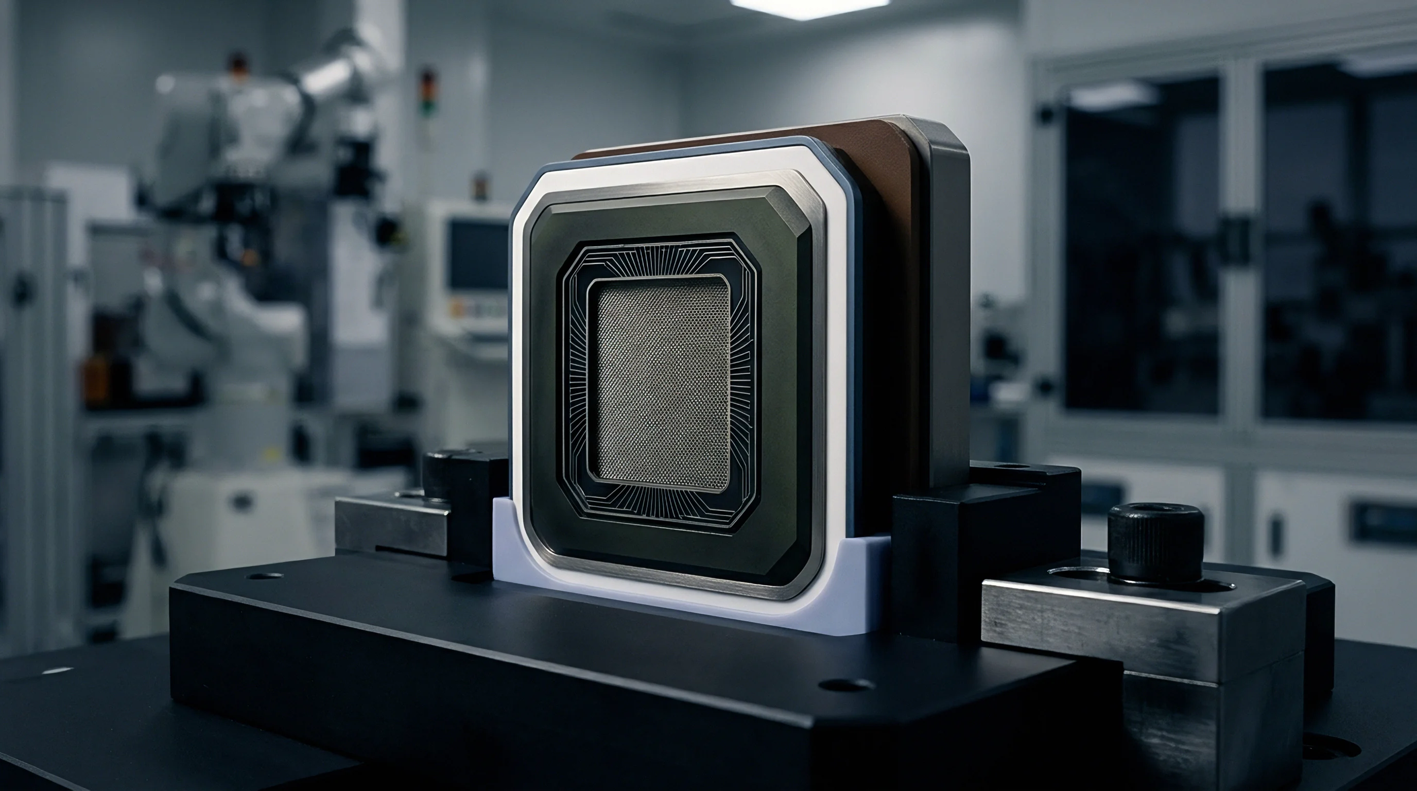
Component datasheets often quote noise density figures taken at room temperature without specifying parameter drift across operating thermal limits. Sensor tier dictates raw component price. Calibration protocols determine final landed unit cost.
A low-cost consumer MEMS accelerometer quoting impressive velocity random walk metrics under static bench conditions may exhibit severe bias shifts when exposed to industrial vibration profiles. Sourcing practices must demand comprehensive factory calibration dossiers or allocate internal capital for automated incoming screening fixtures.
| Sensor Grade Class | Angle Random Walk | Bias Stability | Velocity Random Walk | Typical Unit Cost Range |
|---|---|---|---|---|
| Consumer Electronics Grade | 0.50 to 2.00 deg/hr^0.5 | 20.0 to 100.0 deg/hr | 200 to 1000 ug/Hz^0.5 | 1.50 to 15.00 USD |
| Industrial Automation Grade | 0.10 to 0.50 deg/hr^0.5 | 5.0 to 20.0 deg/hr | 50 to 200 ug/Hz^0.5 | 45.00 to 250.00 USD |
| Tactical Navigation Grade | 0.01 to 0.10 deg/hr^0.5 | 0.5 to 5.0 deg/hr | 10 to 50 ug/Hz^0.5 | 800.00 to 4500.00 USD |
| Navigation Grade (FOG / MEMS) | Under 0.005 deg/hr^0.5 | Under 0.1 deg/hr | Under 5 ug/Hz^0.5 | 8000.00 to 25000.00 USD |
Procuring sensors for safety-critical applications mandates rigorous verification of parameter consistency across production lots. Wafer-level variations cause batch-to-batch discrepancies in comb-structure resonance and damping coefficients. When secondary sourcing requires swapping an IMU model from a secondary vendor, engineering teams must evaluate whether continuous process noise matrix Q_c requires updating.
Mismatched Allan variance profiles between primary and secondary sensor options degrade Kalman filter state estimation accuracy, potentially triggering unexpected system failure modes during field deployment.
- Allan Variance Test Protocol ~ Require suppliers to submit 16-hour static benchmark Allan variance curves per lot, confirming ARW, VRW, and bias stability compliance across ambient temperature ranges.
- Thermal Drift Coefficients ~ Validate third-order polynomial bias-versus-temperature correction parameters provided in sensor non-volatile memory to limit rate random walk expansion.
- Vibration Rectification Limits ~ Mandate factory verification of vibration rectification coefficients under 2g RMS random vibration testing spanning 20 Hz to 2000 Hz.
- Cross-Axis Matrix Deliverables ~ Secure factory-measured 3×3 alignment matrices for each shipped unit to eliminate manual axis alignment procedures on assembly lines.
- Long-Term Lifecycle Guarantees ~ Mandate ten-year component availability commitments and dual-wafer foundry sourcing agreements before approving sensor part numbers for mass production.
Specification under ISO 26262 ASIL-D mandates dual-source qualification with identical noise density parameters, forcing secondary suppliers to match primary Allan variance profiles to avoid recalibrating filter process noise matrices.