Ground Alignment Error Bounds for Inertial Navigation Initialization
Ground alignment error bounds depend on accelerometer turn-on bias for leveling and East gyro bias stability divided by cosine latitude for heading accuracy.

Earth
Ground initialization of an inertial navigation system relies on two physical vectors: local gravity and Earth’s rotation. Accelerometers measure specific force ~ the combined effect of gravity and any translational acceleration ~ while gyroscopes track total angular rate in inertial space. Once the sensor frame sits stationary on the ground, translational kinematic acceleration drops out entirely, leaving gravity as the sole reference for leveling pitch and roll.
At the same time, the planet’s rotation rate of 15.04107 degrees per hour provides the reference vector for true North. Together, these two vectors allow an inertial unit to establish its local coordinate frame without relying on GNSS, radio aids, or optical sightings.
Where the system sits on the planetary ellipsoid dictates how these vectors project onto the instrument axes. Geodetic latitude governs the angle between the local vertical and Earth’s spin axis. At the equator, gravity and planetary spin are perpendicular, providing the strongest horizontal signal for finding true North.
As an instrument moves poleward, the horizontal projection of Earth’s rate falls off with the cosine of latitude, compressing the usable rotation signal into the sensor noise floor. By 80 degrees latitude, this horizontal rate drops to just 2.61 degrees per hour ~ an 82 percent reduction compared to the equator.

Vector Decomposition of Local Gravitational and Rotational Fields
In practice, sensors mounted to a rigid base measure vectors resolved into the local level navigation frame, typically East-North-Up or North-East-Down. In an East-North-Up implementation, gravity acts downward along the negative vertical axis, while the Earth rotation vector lies entirely within the North-Up meridian plane. Resolved mathematically, this vector has a horizontal North component equal to the planetary rate scaled by the cosine of latitude, and a vertical Up component scaled by the sine of latitude.
In a properly aligned East-North-Up frame, the East component is identically zero.
Alignment routines take advantage of that zero-rate condition along the transverse horizontal axis. Any angular rate measured along the East axis during a static hold indicates either a raw sensor bias or an azimuth error relative to true North. By resolving these horizontal rates, the navigation processor solves for the direction cosine matrix between the sensor body and the local level frame.
The ultimate accuracy of this solution depends on how cleanly the triad separates true angular motion from cross-axis mechanical coupling.
At 45 degrees latitude, an uncompensated gyro bias of 0.01 degrees per hour induces an initial heading alignment error of 0.053 degrees.
Frame Rotations and Kinematic Constraints during Stationary Alignment
When an inertial unit is bolted to a stationary vehicle or test stand, its velocity relative to the ground is zero. This zero-velocity condition serves as a rigid kinematic constraint in the navigation equations. Because the base is not translating, accelerometer outputs reflect only the reaction force opposing local gravity.
Pitch and roll can therefore be computed directly from trigonometric ratios of the specific force vector, without integrating velocity over time.
Static initialization runs in two successive steps: coarse vector matching followed by fine filtering. Coarse alignment computes an approximate attitude matrix from cross-products of the raw acceleration and gyro vectors. This runs in a few seconds, establishing a rough coordinate frame with loose error bounds.
Fine alignment then passes this estimate to a multi-state Kalman filter that estimates residual instrument biases, tracks base vibration, and propagates the error covariance. Convergence time is governed by the sensor noise spectral density and the mechanical stability of the mounting surface.
Deflection of the vertical imposes an absolute physical ceiling on leveling accuracy. Subsurface crustal mass anomalies pull the local gravity vector away from the mathematical ellipsoidal normal by several arcseconds. Because stationary accelerometers align strictly with the true gravimetric vector rather than the reference ellipsoid, unmodeled deflections map straight into the attitude matrix as systematic tilt errors that laboratory sensor calibration cannot eliminate.

Drift
Instrument imperfections superimpose parasitic errors onto physical reference signals during ground alignment. Total drift is a compound of deterministic bias offsets, thermal hysteresis, and stochastic noise. Turn-on bias repeatability is usually the largest deterministic hurdle.
Each time an IMU powers up, thermal settling and internal package stresses cause the zero-input bias to land on a new, unpredictable value. While this offset remains relatively stable during a short run, it resets across power cycles.
Stochastic noise corrupts the integration process over the alignment window. Wideband noise in rate gyros creates angle random walk (deg/sqrt(hr)), while accelerometer white noise produces velocity random walk. When integrated, white noise generates an error envelope that expands with the square root of time.
In fine alignment filters, this noise floor sets the minimum duration required to observe and estimate fixed sensor biases with reasonable confidence.
Noise Floor Limits and Stochastic Error Propagation
Flicker noise and low-frequency bias instability define the asymptotic precision limit for ground alignment. Extending static dwell times cannot average out 1/f noise. Once an alignment run reaches the Allan variance bias instability floor, continued averaging yields no improvement in state estimates.
Signal conditioning circuits must therefore balance sampling rates and anti-aliasing filter cutoffs so high-frequency broadband noise does not alias back into the bias instability region.
Analog-to-digital conversion stages inside the IMU add quantisation noise and thermal gain errors. Quantisation noise sets the short-term noise floor whenever converter resolution is coarser than the transducer’s thermal noise. A 24-bit delta-sigma ADC paired with a high-g accelerometer provides plenty of discrete resolution, but reference voltage drift over temperature will still register as false acceleration.
Furthermore, micro-volt thermal EMFs generated across dissimilar PCB trace junctions during warm-up mimic static acceleration shifts on the front-end amplifiers.
| Sensor Modality | Turn-On Bias Repeatability | Bias Instability | Angle / Velocity Random Walk | Analytical Leveling Bound | Azimuth Bound at 45 deg |
|---|---|---|---|---|---|
| Navigation Ring Laser Gyro (RLG) / Quartz Accelerometer | 0.003 deg/hr, 15 micro-g | 0.001 deg/hr, 5 micro-g | 0.002 deg/sqrt(hr), 3 micro-g/sqrt(Hz) | 0.003 mrad | 0.016 deg |
| Tactical Fiber Optic Gyro (FOG) / Silicon MEMS | 0.05 deg/hr, 100 micro-g | 0.01 deg/hr, 25 micro-g | 0.015 deg/sqrt(hr), 20 micro-g/sqrt(Hz) | 0.020 mrad | 0.270 deg |
| High-Grade Tactical MEMS Triad | 0.50 deg/hr, 500 micro-g | 0.10 deg/hr, 50 micro-g | 0.100 deg/sqrt(hr), 100 micro-g/sqrt(Hz) | 0.100 mrad | 2.710 deg |
| Industrial MEMS IMU Modality | 5.00 deg/hr, 2000 micro-g | 1.00 deg/hr, 250 micro-g | 0.500 deg/sqrt(hr), 500 micro-g/sqrt(Hz) | 0.400 mrad | 27.10 deg |

Thermal Trajectories and Dynamic Bias Drift Profiles
Transient thermal gradients across the sensor assembly produce noticeable bias swings during startup. Onboard electronics dissipate heat into ceramic headers, fiber coils, or quartz flexures, driving structural expansion that alters capacitive pickoff gaps or optical path lengths. If left uncorrected, these dynamic thermal shifts mimic true base motion in the static alignment filter.
IMU firmware typically applies multi-order polynomial correction tables stored in EEPROM, driven by temperature sensors mounted directly to the transducer die or optical bench. Thermal hysteresis, however, limits how well open-loop compensation works. During thermal cycling, mechanical stress relaxation rarely follows the exact path seen during warm-up, leaving residual unmodeled bias errors.
Tactical silicon accelerometers subjected to a 20 degree step change in ambient temperature exhibit transient bias excursions up to 180 micro-g before settling at thermal equilibrium.
Several distinct electrical and mechanical mechanisms degrade ground initialization accuracy:
- Thermal Gradient Hysteresis shifts mechanical mounting stress across transducer substrates, creating uncompensated turn-on bias drift during system warm-up.
- Analog Signal Chain DC Offsets inside high-gain preamplifiers corrupt static accelerometer outputs, introducing false horizontal tilt angles in coarse leveling.
- Clock Jitter in Phase-Sensitive Demodulators degrades optical gyro frequency tracking, raising high-frequency phase noise and inflating angle random walk.
- Vibration Rectification Non-Linearity converts ambient mechanical vibration into fictitious DC acceleration through asymmetric flexure suspension compliance.
- Cross-Axis Strain Coupling warps sensor mounting frames under structural torque, causing horizontal angular rates to bleed into vertical channels.
Starting an alignment with uncalibrated sensors corrupts the initial state covariance. When that happens, the filter can diverge rapidly as soon as the vehicle moves.

Tilt
Analytical leveling determines pitch and roll by measuring the specific force components normal to the gravity vector. When stationary, horizontal accelerometers read only the acceleration produced by tilt relative to the local gravimetric horizon. Under small-angle assumptions, pitch is simply the forward specific force divided by gravity, and roll is the lateral force divided by gravity.
The accuracy of these two readings sets the leveling error floor.
Accelerometer turn-on bias maps straight into tilt uncertainty. Dividing horizontal bias by local gravity yields the angular tilt error in radians; for small angles, 1 micro-g of bias produces roughly 1 micro-radian of tilt error. A tactical-grade accelerometer with a 100 micro-g turn-on bias therefore imposes a hard leveling limit of 0.1 milliradians (about 20 arcseconds), no matter how long the static filter runs.
Accelerometer Bias Calibration and Leveling Precision Bounds
Horizontal tilt error propagation during static leveling is governed by straightforward error dynamics. Pitch error δ thη and roll error δ φ depend on turn-on bias ba, scale factor error Sa, cross-axis alignment angle α, and broadband noise na according to:
δ thη = fracbaxg + Sax thη + αxy φ + fracnaxg sqrtT
δ φ = -fracbayg – Say φ – αyx thη – fracnayg sqrtT
Scale factor errors become significant when leveling on inclined ground. On a 15-degree slope, a 500 ppm accelerometer scale factor uncertainty produces an effective error proportional to gravity times the sine of 15 degrees times 500 ppm. This yields 130 micro-g of apparent bias, adding 26 arcseconds of leveling error.
Without accurate scale factor calibration, static leveling on slopes degrades quickly.
Horizontal accelerometer bias sets the absolute leveling threshold, whereas gyro noise dictates the time required to settle at that threshold.
Horizontal Accelerometer Cross-Axis Coupling and Mounting Misalignment
Internal package misalignments introduce parasitic cross-axis coupling. If the sensing axes are not strictly orthogonal, the full 1 g gravitational field sensed on the vertical channel bleeds into the horizontal channels. With an orthogonality error of 0.1 milliradians, vertical gravity projects an apparent 981 micro-g offset onto the horizontal axis.
That uncalibrated coupling produces a tilt error nearly ten times larger than the native turn-on bias of a navigation-grade accelerometer.
Multi-position factory calibration routines correct for these non-orthogonality matrices under static conditions, mapping misalignment terms down to arcsecond thresholds. However, installing the IMU onto a vehicle chassis introduces new mechanical strain. Fastener torque distorts the baseplate, shifting internal alignment away from factory calibration.
Isolation mounts help damp high-frequency vibration, but they also introduce low-frequency mechanical sag that shifts with vehicle loading.
Static filters must isolate these structural tilt errors before feeding attitude data to the heading estimator. Any residual tilt error projects vertical Earth rate into the horizontal gyro channels, directly biasing the azimuth solution.
Levelling accuracy improves when static integration time matches the environmental noise spectrum.
Heading
Gyrocompassing determines true North by measuring the horizontal component of Earth’s rotation. When leveled, a horizontal gyroscope pointing true East senses zero planet rotation. Sweeping that gyro axis toward North increases the measured rate until it peaks on the meridian.
Alignment routines adjust the estimated heading until the measured rate on the East-facing gyro nulls out completely.
Gyro bias stability sets the baseline heading accuracy. Any uncompensated bias on the East horizontal channel looks like Earth rotation, forcing the estimator to compute a false heading offset to balance it. The heading error δ ψ caused by an East gyro bias bge is a function of Earth’s rate Ωe and geodetic latitude φ:
δ ψ = fracbgeΩe cosφ
Horizontal accelerometer bias also introduces heading error through leveling errors. An uncorrected pitch or roll tilt tilts the horizontal frame relative to gravity, projecting the vertical component of Earth rate onto the East-West gyro. Accounting for accelerometer bias bax yields the combined heading error expression:
δ ψtotal = fracbgeΩe cosφ + fracbaxg tanφ
Analytic Gyrocompassing Equations and Latitude Singularities
Heading error increases rapidly as the system moves away from the equator. The secant latitude term scales any residual gyro bias: the multiplier is 1.0 at the equator, doubles to 2.0 at 60 degrees latitude, and reaches 11.47 at 85 degrees. Near the poles, minor gyro biases translate into multi-degree heading errors.
| Geodetic Latitude | Horizontal Earth Rate Component | FOG Nav-Grade Heading Error (0.005 deg/hr bias) | MEMS Tac-Grade Heading Error (0.1 deg/hr bias) | Required Fine Alignment Time (Nav Grade) | Required Fine Alignment Time (Tactical Grade) |
|---|---|---|---|---|---|
| 0 degrees (Equator) | 15.041 deg/hr | 0.019 deg | 0.381 deg | 180 sec | 1200 sec |
| 30 degrees | 13.026 deg/hr | 0.022 deg | 0.440 deg | 240 sec | 1500 sec |
| 45 degrees | 10.636 deg/hr | 0.027 deg | 0.539 deg | 360 sec | 2100 sec |
| 60 degrees | 7.521 deg/hr | 0.038 deg | 0.762 deg | 600 sec | 3600 sec |
| 75 degrees | 3.893 deg/hr | 0.074 deg | 1.472 deg | 1200 sec | 7200 sec |

When Does Dynamic Base Motion Overwhelm Static Alignment Filters?
Base motion degrades ground alignment when vehicle motion violates the static noise assumptions built into the Kalman filter. Wind buffeting the chassis, engine idle vibration, footsteps on deck, or cargo handling introduce motion signals that dwarf Earth’s rotation rate. If a static filter interprets these external motions as pure sensor noise, covariance estimates diverge and bias estimation fails.
Running coarse vector matching prior to fine Kalman filtering stabilizes initialization against these base disturbances. A standard sequence for reliable field alignment involves:
- Sample stationary multi-axis accelerometer and gyroscope channels continuously over a two-second sliding baseline to compute local noise variance statistics.
- Reject initial data frames if high-g mechanical transient shocks exceed five times expected ambient floor levels.
- Compute coarse pitch and roll angles by averaging specific force vectors across a twenty-second stationary integration frame.
- Form initial coordinate transformation matrices matching measured gravity and rough spatial orientation.
- Estimate coarse heading by evaluating transverse horizontal angular rate cross-products relative to transformed gravitational axes.
- Initialize Kalman filter state vector covariance matrices using calculated coarse attitude uncertainties and published sensor turn-on repeatability parameters.
- Execute multi-state Extended Kalman Filtering using zero-velocity and zero-rate update constraints to refine bias estimates and converge on final azimuth angle.
Convergence time depends primarily on angle random walk. Low-noise ring laser gyros average out broadband noise quickly, converging on azimuth within minutes. Higher-noise MEMS units need longer static integration windows to separate planetary rotation from the integrated noise floor.
If an alignment is cut short before the filter covariances settle, residual heading uncertainty scales directly with the unestimated bias variance.
Distinguishing weak polar rotation rates from low-frequency structural thermal expansion remains a central challenge for adaptive filtering during extended static initialization at high latitudes.
Disturbance
Environmental disturbances complicate alignment by breaking the core assumption of zero base motion. Diesel engine idle, industrial equipment nearby, wind loads, and ground vibrations all create oscillatory accelerations far larger than static gravity. When high-frequency vibration excites structural resonances, accelerometer vibration rectification transforms symmetric AC vibrations into artificial DC bias shifts via suspension non-linearities.
Angular base motion is especially problematic because vehicle rocking can produce rates thousands of times greater than Earth’s rotation. Wind buffeting a tall vehicle chassis easily generates sway rates of several degrees per second between 0.2 and 1.5 Hz. Filtering algorithms must attenuate these sway frequencies without adding phase lag that distorts attitude updates.

Vibration Rectification and Angular Base Disturbance Spectral Noise
Vibration rectification occurs in MEMS and quartz flexure accelerometers when non-linear spring stiffness or asymmetric squeeze-film damping distorts the response to harmonic inputs. Under broadband random vibration, the sensor rectifies high-frequency energy into a steady-state DC bias shift Δ bvre:
Δ bvre = Kvre · grms2
The vibration rectification coefficient Kvre (expressed in micro-g per g2rms) varies substantially by transducer design. Tactical MEMS accelerometers with asymmetrical beam stops can have rectification coefficients reaching 100 micro-g/g2rms. Under a typical 1.5 grms engine idle profile, this non-linearity generates an apparent 225 micro-g DC shift.
That bias adds 0.22 milliradians of leveling error, overshadowing the sensor’s native turn-on repeatability.
Under MIL-STD-810H vibration exposures, unfiltered angular base motion induces non-linear gyro rectification drifts that double the residual heading uncertainty.
Adaptive Filtering Mechanics for Transient Base Displacement Rejection
To maintain filter stability under transient base motion, practical estimators adaptively scale the measurement noise covariance matrix Rk. When onboard shock sensors or residual monitoring routines detect an anomalous acceleration spike, the filter inflates the diagonal elements of Rk. This temporarily lowers the Kalman gain, preventing transient shocks from corrupting the core navigation states.
Choosing effective disturbance rejection thresholds requires matching the operational profile to sensor dynamics:
- Spectral Bandwidth Separation isolates high-frequency mechanical engine vibration from low-frequency base motion using sharp-cutoff digital Butterworth low-pass filters.
- Adaptive Innovation Thresholding monitors Kalman filter residual sequences, zeroing measurement updates when transient base motion exceeds three standard deviations.
- Wavelet Denoising Decomposition separates non-stationary transient shock spikes from underlying static Earth rate signal components in high-vibration operational zones.
- Dual-Antenna GNSS Vector Aiding provides independent coarse heading constraints during ground alignment when extreme mechanical base sway overwhelms static gyrocompassing solvers.
Chassis vibration during engine idle is frequently assumed to stay within published white-noise bounds, but non-linear rectification inside the transducer housing introduces steady DC bias offsets that bypass simple averaging.

Bench
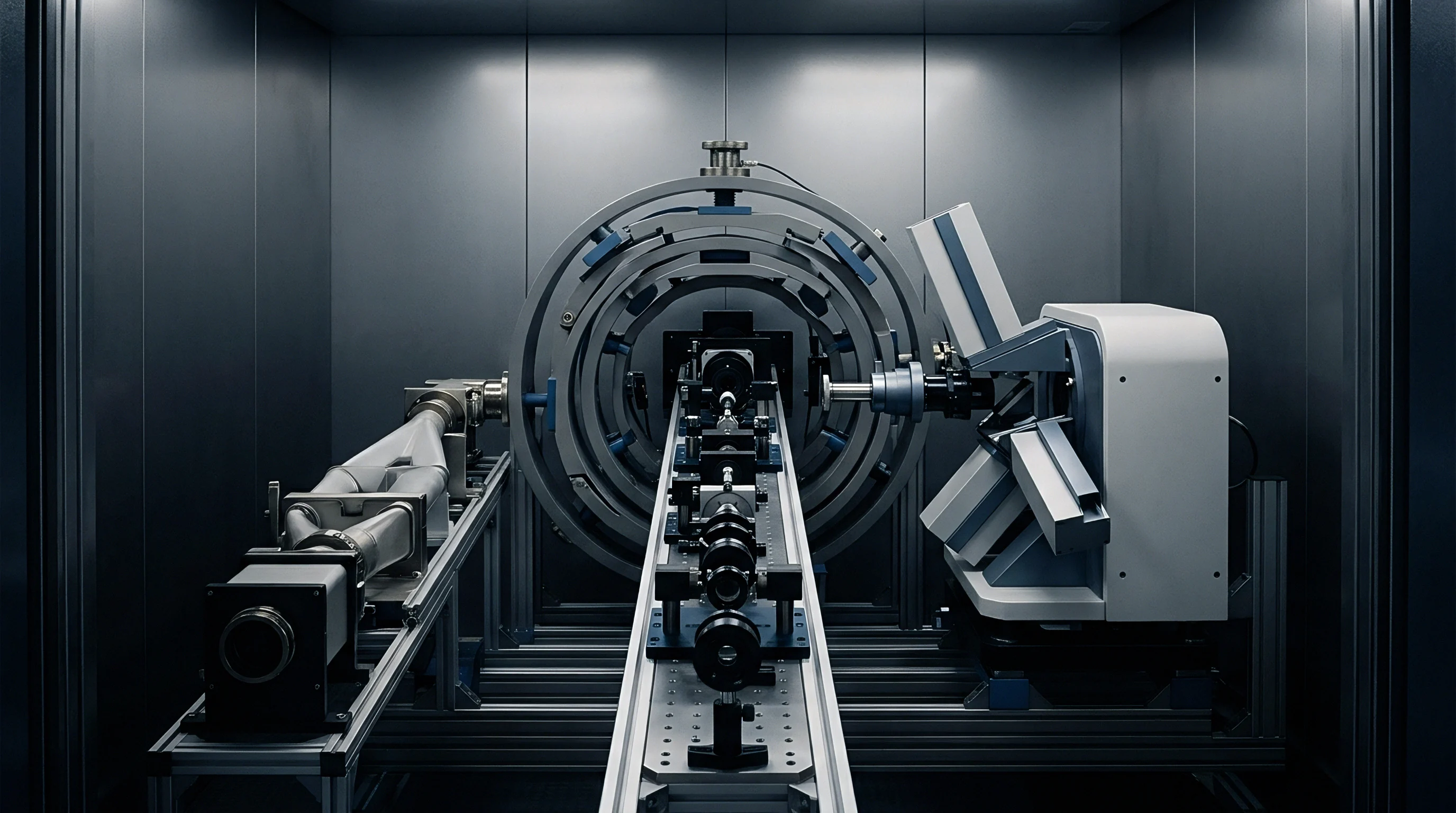
Validating ground alignment error budgets requires multi-axis rate tables and static tilt fixtures. Laboratory testing checks that sensor triads meet published specifications for bias repeatability, noise floor, and axis orthogonality under controlled conditions. Standards such as IEEE 1554, IEEE 952, and IEEE 1431 outline specific static tilt and rate test profiles.
These protocols call for thorough thermal soaking, optical encoder tracking, and seismically isolated test foundations to keep ambient laboratory vibrations out of the dataset.
Multi-position static indexing isolates accelerometer turn-on bias from cross-axis coupling and gravity anomalies. By stepping an IMU through a series of known orthogonal orientations, test software builds a system of linear equations that separates scale factor errors, mounting misalignment, and raw zero-input bias. A standard 12-position tumble test positions each axis at 0, 90, 180, and 270 degrees relative to gravity, allowing matrix solvers to resolve calibration parameters down to the single micro-g level.
Multi-Position Indexing and Static Laboratory Tilt Calibration Protocols
Two-axis indexing mounts evaluate gyrocompassing without requiring hours of static dwell time. Rotating an IMU 180 degrees about its vertical axis reverses the sign of Earth rate sensed on the horizontal gyros while leaving internal sensor biases unchanged. Taking the difference between these two measurements doubles the apparent Earth rate signal and cancels the constant gyro bias.
Using this indexing technique during field startup allows tactical-grade sensors to deliver heading performance close to that of expensive navigation-grade optical gyros.
Testing must also account for chamber noise. Compressor and blower vibration inside standard environmental test chambers generates high-frequency mechanical noise that distorts turn-on bias measurements. High-accuracy qualification requires thermally quiet chambers chilled with liquid nitrogen or remote ducting to keep ambient vibration below 100 micro-g across the 10 Hz to 2 kHz band.
| Transduction Technology | Substrate / Active Material | Turn-On Bias Repeatability | Reachable Azimuth at 10 Minutes | Unit Cost Range (USD) | Single-Source Supply Exposure |
|---|---|---|---|---|---|
| Monolithic Quartz Flexure Accelerometer | Etched Fused Quartz Crystal | 10 to 30 micro-g | 0.015 to 0.030 deg (with RLG) | $3,500 – $8,000 | High (Limited global wafer foundries) |
| High-Performance MEMS Capacitive Accelerometer | Deep Reactive-Ion Etched Silicon | 100 to 300 micro-g | 0.150 to 0.500 deg (with FOG) | $400 – $1,200 | Moderate (Multiple commercial MEMS fabs) |
| Ring Laser Gyroscope (RLG) Triad | Zero-Expansion Glass Ceramic (Zerodur) | 0.002 to 0.008 deg/hr | 0.010 to 0.025 deg | $25,000 – $60,000 | High (Specialized optical fabrication) |
| Closed-Loop Fiber Optic Gyroscope (FOG) | Polarization-Maintaining Optical Fiber | 0.020 to 0.100 deg/hr | 0.050 to 0.200 deg | $8,000 – $22,000 | Moderate (Widespread fiber optic winding) |
| Tactical Silicon MEMS Gyroscope Triad | Polysilicon Quad-Mass Resonator | 0.200 to 1.500 deg/hr | 0.800 to 3.000 deg | $800 – $3,500 | Low (Broad commercial supplier base) |

Commercial Sourcing Tiers and Unit Cost Dynamics across Sensor Modalities
Selecting inertial hardware requires trading physical performance against lifecycle cost and supply continuity. Systems requiring sub-arcminute heading in under a few minutes rely on Ring Laser Gyros (RLGs) or closed-loop Fiber Optic Gyros (FOGs). These optical sensors provide exceptional bias stability and very low angle random walk, but unit prices regularly exceed $20,000.
Producing them requires high-vacuum optical cavity sealing, precise glass machining, and specialized fiber coil winding ~ capabilities concentrated among a handful of defense suppliers.
Tactical silicon MEMS IMUs offer substantial cost, size, and power advantages, along with higher shock tolerance. However, their higher angle random walk limits standalone static gyrocompassing. Getting useful heading accuracy from MEMS hardware usually requires software aiding, indexing mechanisms, or longer alignment windows.
When second-sourcing MEMS parts, engineering teams must carefully qualify thermal coefficients, die attach stresses, and long-term bias stability across foundries.
Batch-to-batch turn-on bias in silicon sensors can vary by up to 40 percent due to minor differences in package resin cure stresses. Because of these packaging variations, an alignment filter tuned for one wafer lot can fail acceptance tests on the next unless every production unit undergoes comprehensive thermal calibration.
A dual-axis indexing mount isolates gyroscope turn-on bias from Earth rate measurement without requiring an external optical reference.
Procurement specifications for navigation-grade units typically require rigorous compliance testing:
Standard qualification clauses specify that turn-on bias repeatability must be calculated as the standard deviation of zero-input signal means measured across twenty consecutive power cycles, with minimum thirty-minute thermal soak periods between cycles, enforced under IEEE 1554 test conditions.