Silicon Pressure Sensor Encapsulation Media Tradeoffs and Calibrations
Sensor media isolation dictates lifecycle drift, requiring matched fill fluid volume and multi-point thermal calibration to hold industrial accuracy.

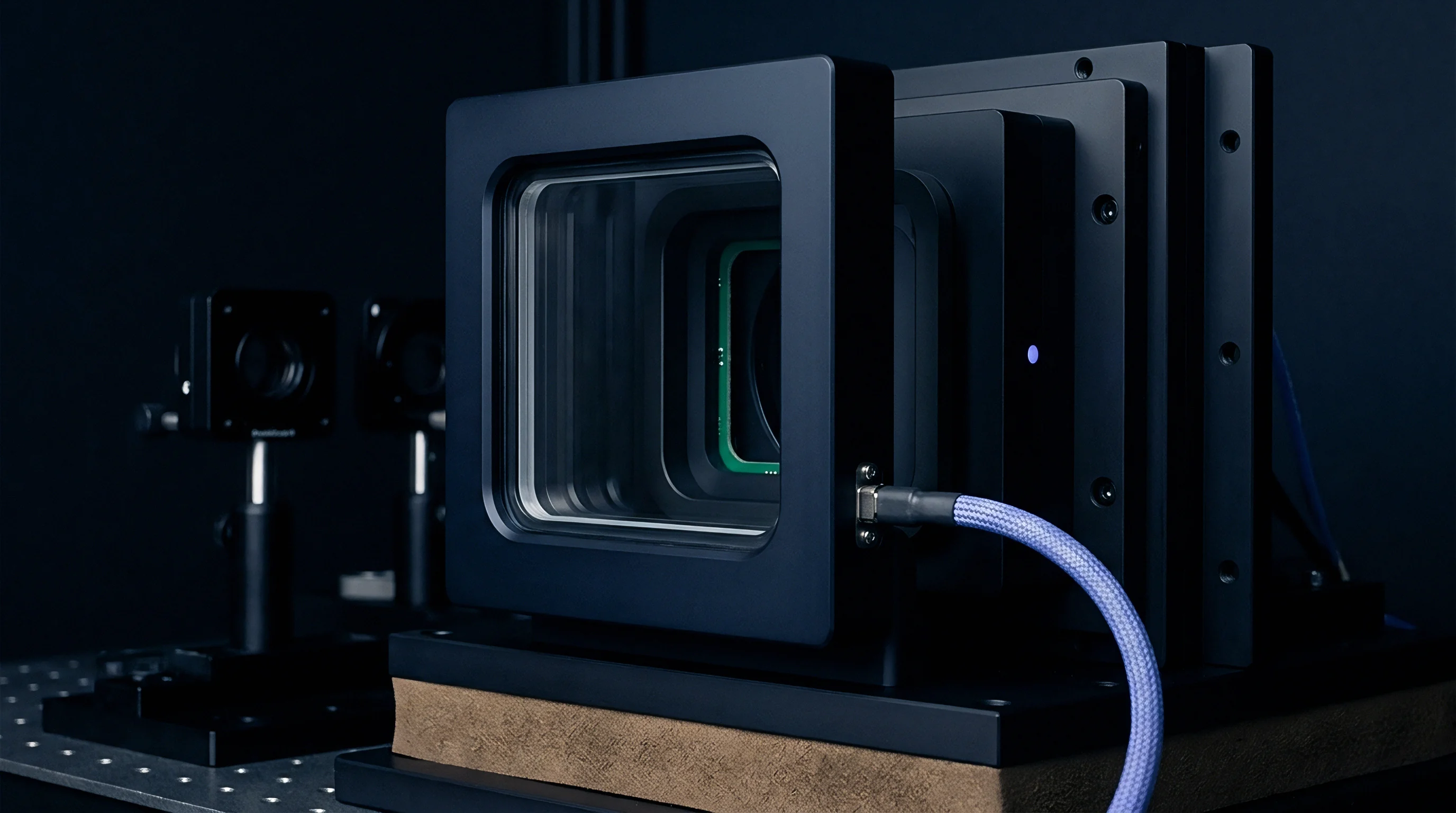
Barrier
Direct exposure of a piezoresistive silicon die to process fluids causes catastrophic electrical shorting, chemical etching of aluminum metallization, or mechanical fracture from suspended particulate. Isolating the micromachined membrane requires a secondary transmission barrier. This barrier couples line pressure to the sensing element while arresting corrosive species, ionic contaminants, and polar molecules.
Sourcing engineers encounter four dominant isolation topologies across commercial pressure transmitters: direct organic coatings, fluorosilicone or silicone gel pots, oil-filled welded metal diaphragms, and back-side absolute cavity mounts.
Piezoresistive die architectures employ diffused or ion-implanted p-type resistors within an n-type silicon diaphragm. Electrical isolation between the Wheatstone bridge resistors and the bulk substrate relies on reverse-biased p-n junctions. Any conductive liquid contacting the top surface shunts these junctions.
Water with ionic content above 5 microsiemens per centimeter induces leakage currents exceeding 20 microamperes, collapsing bridge sensitivity and generating offset errors that exceed 15 percent of full scale span within hours of deployment.
A bare silicon diaphragm exposed to humid industrial air drifts beyond its full-scale span tolerance within forty-eight hours of ionic condensation.
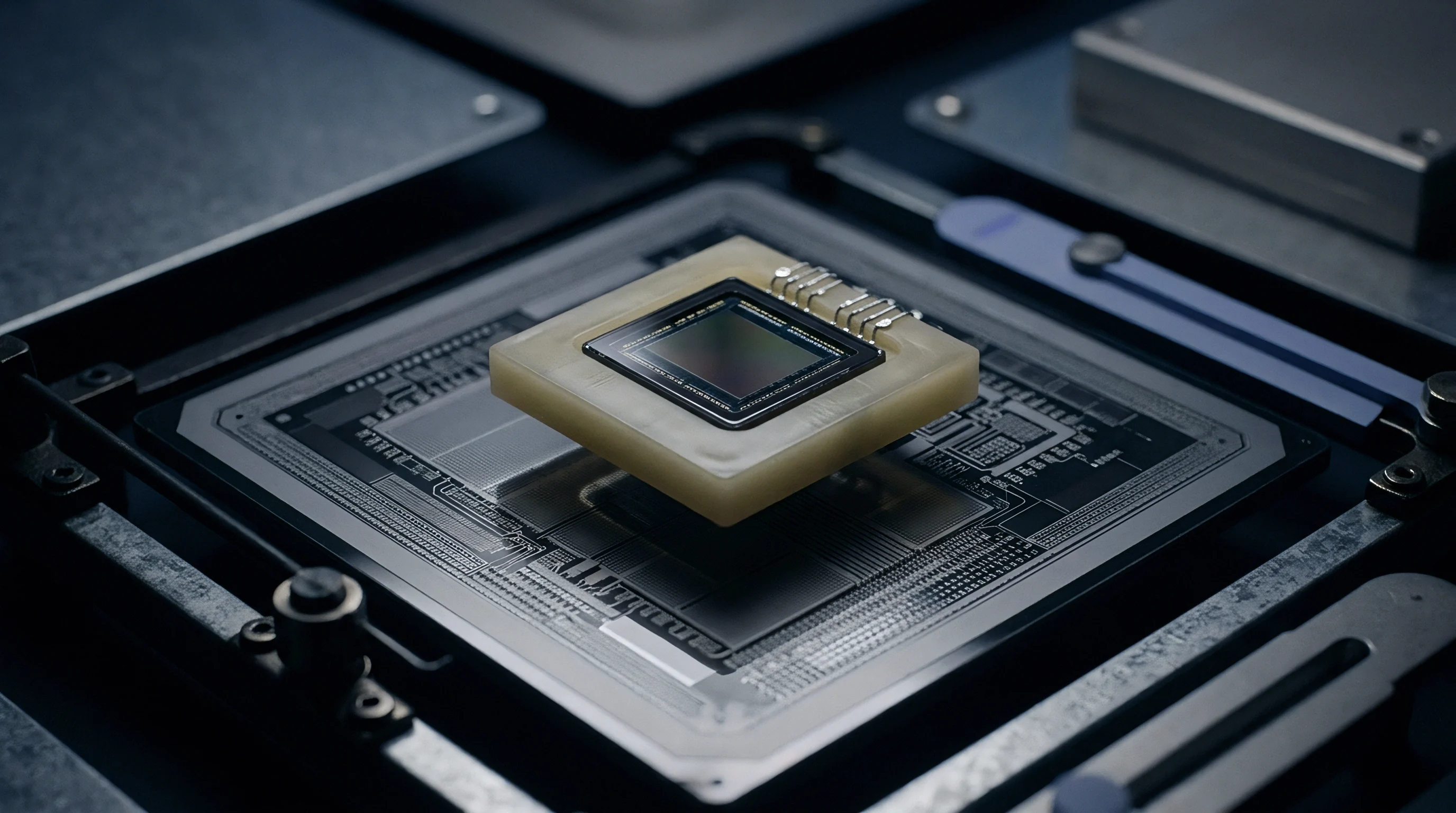
Organic passivation layers such as vapor-deposited Parylene C provide conformal pinhole-free coverage at thicknesses between 2 and 5 micrometers. These films protect against moisture condensation and mild chemical vapor. They perform reliably across non-condensing industrial automation lines, pneumatic manifolds, and HVAC filtration monitoring.
Parylene C exhibits a low dielectric constant of 3.1 at 1 kilohertz and high dielectric breakdown strength of 267 kilovolts per millimeter. The deposition process occurs at room temperature inside a vacuum chamber, preventing thermal stress accumulation across the micromachined silicon edges.
Thin polymer films possess mechanical stiffness that degrades sensor sensitivity when deposited too thick. A 5-micrometer layer of Parylene C on a 10-micrometer-thick silicon membrane reduces raw pressure sensitivity by 6 to 11 percent while introducing an uncompensated temperature coefficient of sensitivity between minus 0.04 and minus 0.08 percent of span per degree Celsius. The mismatch between the thermal expansion coefficient of Parylene C at 35 parts per million per Kelvin and silicon at 2.6 parts per million per Kelvin creates baseline thermal hysteresis.
Temperature cycling from minus 40 to plus 85 degrees Celsius generates zero-return errors reaching 0.35 percent of full scale span.

Mechanical Properties of Barrier Layers
Elastomeric encapsulation provides physical isolation without restricting volumetric displacement. Low-modulus silicone gels distribute hydrostatic pressure equally across the die surface. The mechanical properties of the primary barrier chemistries dictate signal fidelity, damping behavior, and baseline drift under temperature cycling.
| Barrier Material | Elastic Modulus (MPa) | Thermal Expansion (ppm/K) | Density (g/cm³) | Useful Range (°C) |
|---|---|---|---|---|
| Silicon Substrate (Reference) | 130,000 to 170,000 | 2.6 | 2.33 | -55 to 150 |
| Parylene C | 2,800 to 3,200 | 35.0 | 1.29 | -40 to 100 |
| Dielectric Silicone Gel | 0.01 to 0.05 | 300.0 | 0.97 | -50 to 180 |
| Fluorosilicone Gel | 0.02 to 0.08 | 280.0 | 1.25 | -40 to 150 |
| AISI 316L Stainless Steel | 193,000 | 16.5 | 8.00 | -60 to 300 |
| Hastelloy C-276 | 205,000 | 11.2 | 8.89 | -100 to 400 |
Oil-filled capsules isolate the silicon chip inside a hermetic subassembly. A thin convoluted metallic diaphragm welded to an outer header isolates an internal cavity filled with high-purity synthetic fluid. Silicone oils such as polydimethylsiloxane, fluorinated fluids like halocarbon oils, or synthetic hydrocarbon isomers transfer hydraulic pressure to the die.
The isolation diaphragm must absorb entire fluid volume shifts across the operational thermal envelope. Hastelloy C-276 and 316L stainless steel serve as standard diaphragm materials. This architecture provides comprehensive media compatibility across hydrocarbon refining, chemical dosing lines, and subsea pipelines.
Welded metal diaphragm subassemblies introduce fixed production costs that shift minimum purchasing thresholds. A bare surface-mount piezoresistive element costs between 1.50 and 4.00 dollars at volumes of 50,000 units. Adding a laser-welded, vacuum-backfilled 316L capsule raises piece-part cost to 18.00 to 34.00 dollars.
Sourcing teams paying for high-grade metallurgy buy immunity against hydrogen embrittlement, galvanic corrosion, and active solvent attacks. Sourcing mistakes here yield permanent zero drift when corrosive media perforates non-metallic seals in service.
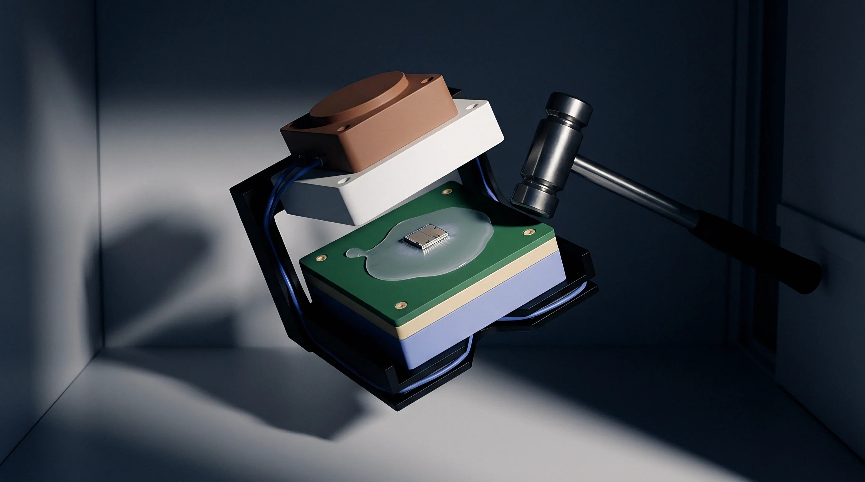
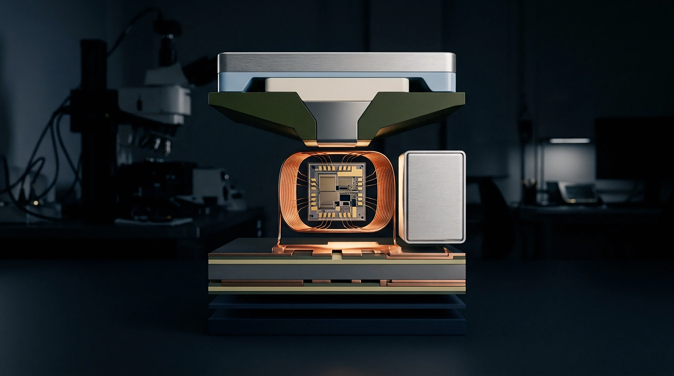
Fill
Hydraulic coupling fluids inside isolated pressure cells introduce thermal, mechanical, and dynamic error mechanisms. The internal fill volume behaves as an expansive thermal body constrained by the spring rate of the metallic isolation diaphragm. Polydimethylsiloxane oils expand significantly across standard industrial temperatures.
An internal fill volume of 0.15 cubic centimeters expanding against a corrugated 316L diaphragm of 12-millimeter diameter generates an internal tare pressure. This hydraulic tare acts directly on the piezoresistive element, registering as zero shift.
The volumetric thermal expansion coefficient of silicone oil sits between 0.00095 and 0.00108 per Kelvin. A transmitter calibrated at 20 degrees Celsius and operated at 70 degrees Celsius experiences a temperature increase of 50 Kelvin. The internal fill oil expands by 4.7 to 5.4 percent of its volume.
If diaphragm stiffness equals 0.8 bar per cubic millimeter, this expansion shifts the zero point by several millibars. In low-range sensors rated below 500 millibar, thermal expansion of the fill fluid accounts for over 70 percent of total uncompensated zero error.

Hydraulic Liquid Formulations
Selecting a fill medium involves balancing chemical stability against kinematic viscosity and thermal expansion. Viscosity dictates response time, especially at freezing temperatures where thick fluids choke hydraulic transmission channels.
- Polydimethylsiloxane Fluid maintains a thermal expansion rate of 0.00096 per Kelvin with kinematic viscosity of 10 centistokes at 25 degrees Celsius, serving inert gas and general industrial hydraulic monitoring.
- Fluorinated Halocarbon Fluid prevents oxidation and ignition in enriched oxygen systems, though it exhibits higher density near 1.9 grams per cubic centimeter and causes hydrostatic orientation errors when sensors rotate.
- High-Purity Mineral Fluid complies with FDA requirements for sanitary food, dairy, and beverage processing lines, operating across a constrained thermal window between minus 10 and plus 85 degrees Celsius.
- Low-Viscosity Silicone Fluid features 5 centistokes viscosity to prevent low-temperature response choking down to minus 45 degrees Celsius, though it exhibits higher evaporation rates during high-vacuum manufacturing.
Hydrostatic head pressure inside the fill cavity imposes an orientation sensitivity that users observe during installation. When a transmitter mounts horizontally rather than vertically, the column height of fill liquid shifts relative to the piezoresistive membrane plane. For halocarbon oil with a density of 1.85 grams per cubic centimeter resting over a 15-millimeter hydraulic path, reorienting the sensor 90 degrees induces a baseline pressure shift of 0.27 millibar.
High-precision calibrations must specify the physical mounting plane relative to gravity. Without this detail, laboratory verification figures diverge from bench-test acceptance thresholds.
Internal fill oil volumes undergo micro-bubble outgassing if vacuum filling fails to achieve deep absolute pressures below 0.01 millibar. Entrained micro-bubbles introduce volumetric compliance into the hydraulic core. This compliance manifests as dynamic lag and non-linear compression profiles under rapid pressure transients.
A capsule with 0.05 percent entrained air by volume shows a pressure response delay reaching 14 milliseconds, compared to 0.8 milliseconds for a properly degassed cell. In high-frequency hydraulic monitoring, compliance dampens transient spikes, blinding monitoring nodes to destructive pressure transients.
Degassing fill fluid below 0.01 millibar during vacuum backfilling remains necessary to prevent non-linear hydraulic compliance under fast pressure pulses.
Viscosity shifts directly determine response times at sub-zero temperatures. Standard 50-centistoke silicone oil thickens to more than 400 centistokes at minus 40 degrees Celsius. Viscous drag through the internal channels linking the metal diaphragm to the chip face delays step-response settling times from 1.2 milliseconds at room temperature to more than 85 milliseconds at minus 40 degrees Celsius.
Systems requiring active closed-loop pressure relief risk over-pressurization when sensor response lags because of low-temperature fluid thickening. Sourcing documents must define maximum response time across the entire thermal envelope rather than quoting ambient 25-degree baseline numbers.
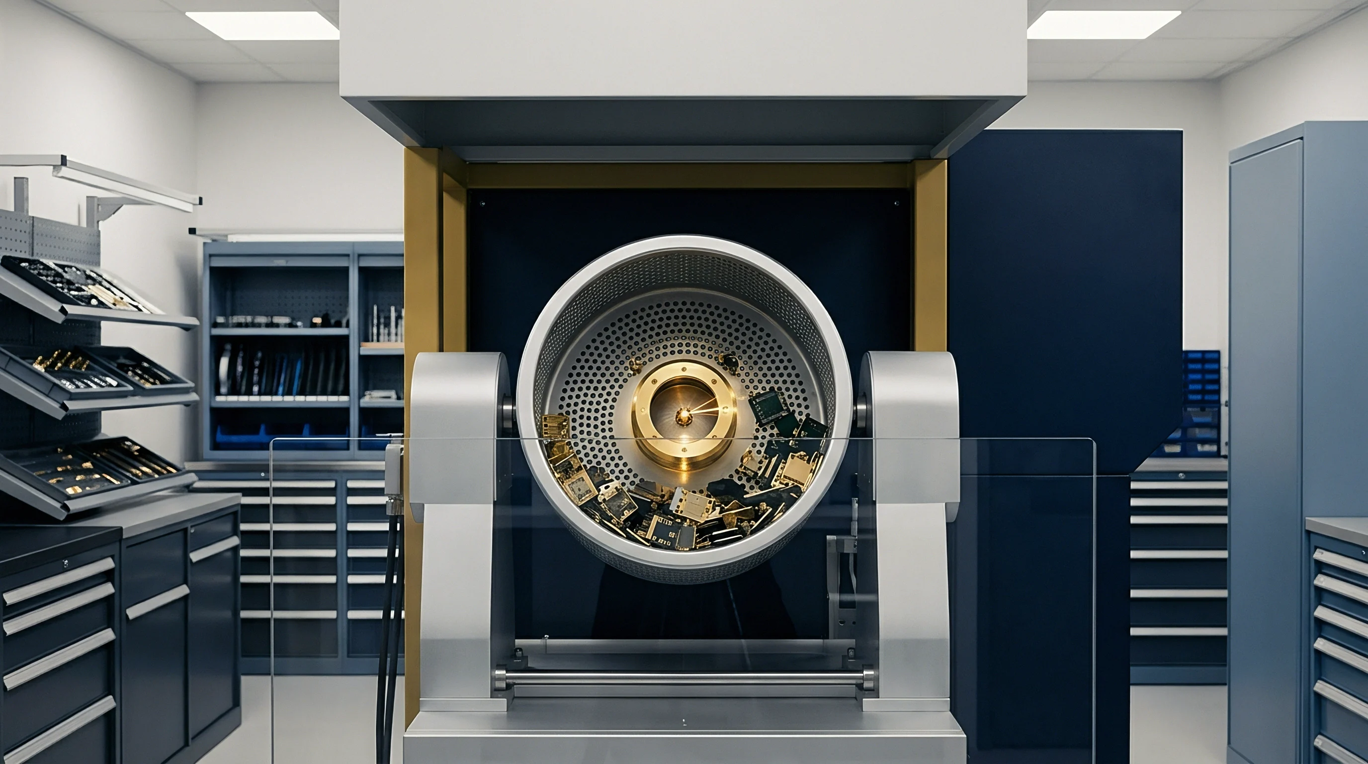
A supplier will often attribute low-temperature sluggishness to host communication processing rather than admitting the fill fluid selected possesses excessive kinematic viscosity at sub-zero baselines.
Swell
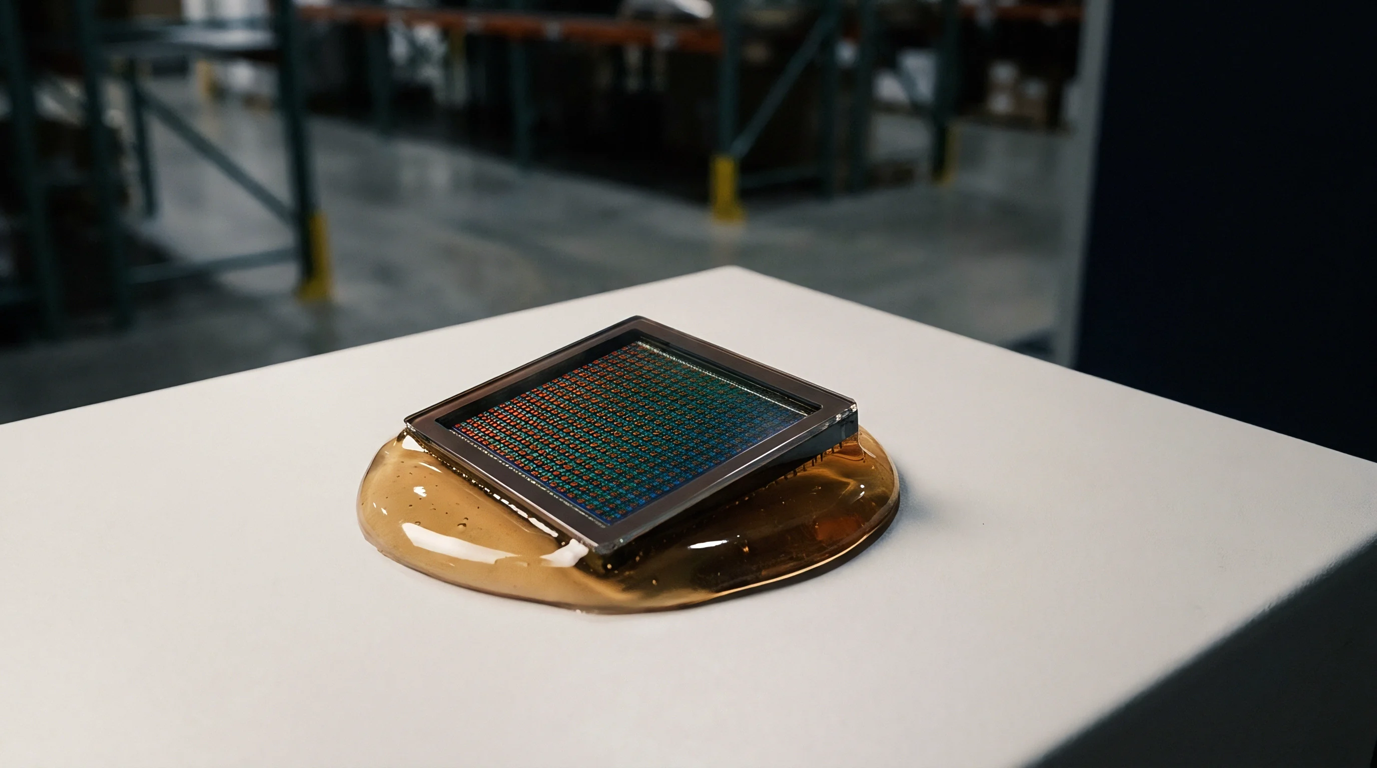
Potted elastomeric encapsulants interact chemically with target media via adsorption and bulk swelling. While low-modulus gels insulate wire bonds and silicon surfaces from trace moisture, organic solvents and polar compounds penetrate the polymer mesh. Cross-linked silicone matrices contain intermolecular voids that admit aliphatic hydrocarbons, aromatic solvents, and volatile organic compounds.
Dissolved solvent molecules dilate the polymer matrix, exerting three-dimensional mechanical strain onto the perimeter of the micromachined silicon die.
Bulk swelling creates compressive stress fields across the chip. Piezoresistors positioned near diaphragm margins possess high piezoresistive coefficients to maximize sensitivity to pressure-induced flexure. Extraneous lateral stress from swelling encapsulants induces large resistance shifts indistinguishable from applied line pressure.
Silicone gels exposed to gasoline, toluene, or diesel fuel experience volumetric swell between 15 and 80 percent within 100 hours. This swelling lifts wire bonds, strips aluminum trace metallization, and causes catastrophic baseline offsets exceeding 30 percent of full scale span.
Permeation and Solvent Resistance
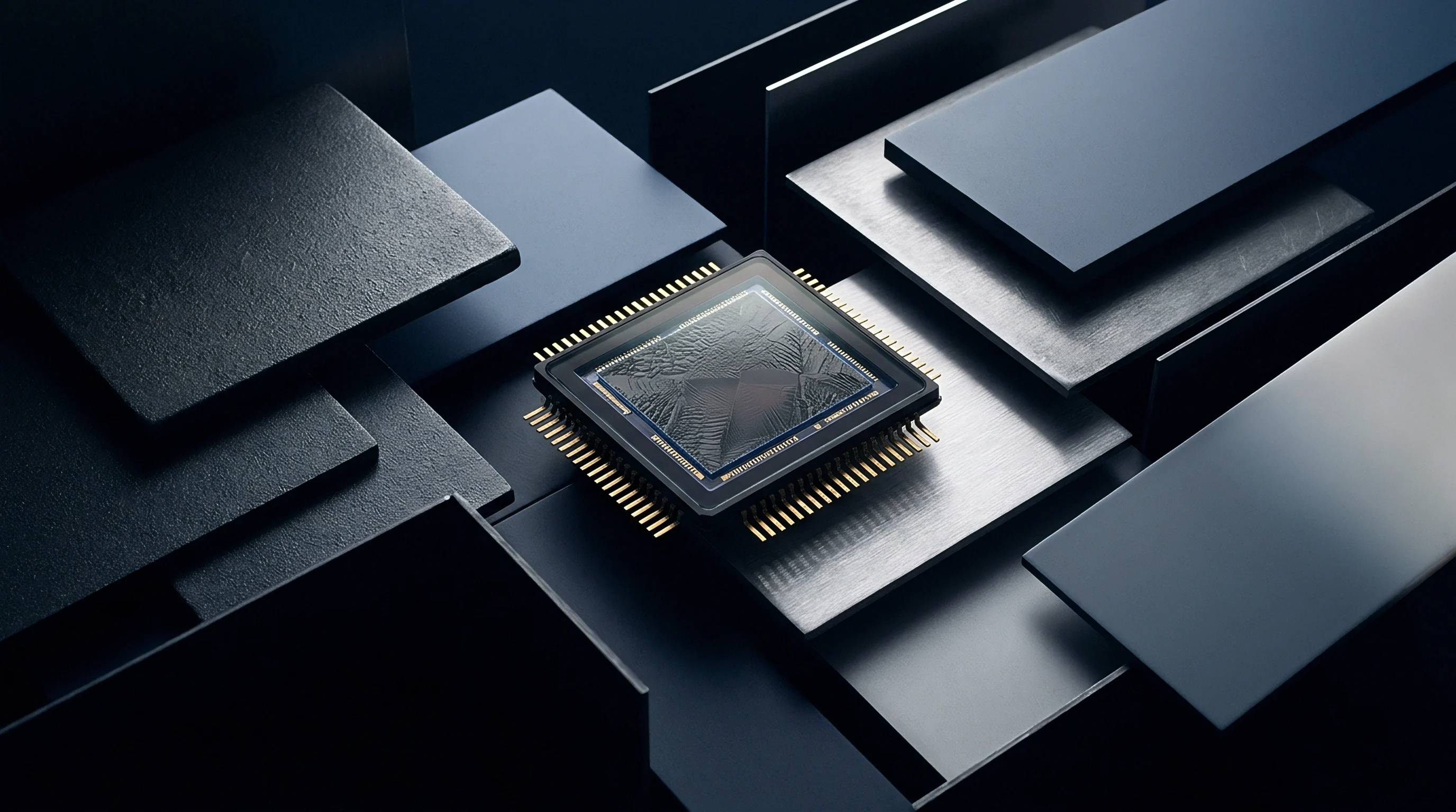
Fluorosilicone polymers improve solvent resilience over standard dimethylsiloxane chemistries. Trifluoropropyl groups along the polymer backbone reduce vulnerability to non-polar hydrocarbons. Fluorosilicones swell less than 5 percent in fuel and oil contact scenarios, maintaining functional stress transmission across automotive powertrain and industrial pump applications.
They exhibit higher glass transition temperatures near minus 60 degrees Celsius, compared to minus 120 degrees Celsius for standard silicones, limiting their elasticity at extreme low temperatures.
| Polymer Chemistry | Test Medium | Exposure (Hours) | Volumetric Swell (%) | Zero Drift (% FSS) |
|---|---|---|---|---|
| Dimethylsilicone Gel | Deionized Water | 1,000 | 0.8 | +0.15 |
| Dimethylsilicone Gel | Diesel Fuel (EN 590) | 168 | 42.5 | +18.40 |
| Fluorosilicone Gel | Diesel Fuel (EN 590) | 168 | 3.1 | +0.85 |
| Fluorosilicone Gel | Engine Coolant (50/50 Glycol) | 1,000 | 1.4 | -0.30 |
| Parylene C | Engine Coolant (50/50 Glycol) | 1,000 | 0.2 | -0.05 |
| Polyurethane Potting | Hydraulic Oil (ISO VG 46) | 500 | 8.6 | +4.20 |
Moisture diffusion through potting formulations drives long-term zero wandering. Water vapor migrates through room-temperature-vulcanized silicones down concentration gradients, condensing at the polymer-die boundary. Water vapor transmission rates through silicone exceed 20 grams per square meter per day at 38 degrees Celsius and 90 percent relative humidity.
Once moisture pools at the silicon dioxide passivated surface, stray DC biases induce electrochemical migration of bond-pad metallization. Gold-aluminum wire bond interfaces form galvanic cells that generate intermetallic voiding, known as Kirkendall voids, which elevate contact resistance and create intermittent open-circuit faults.
Thermal excursions induce significant volumetric shifts inside unconstrained potted cavities. Silicone elastomeric compounds have volumetric thermal coefficients of expansion around 300 to 900 parts per million per Kelvin. The surrounding plastic, ceramic, or metallic housing expands at 5 to 25 parts per million per Kelvin.
Rising ambient temperature forces the gel upward against the housing walls. The resulting shear stresses pull on bonded gold wires measuring 25 to 32 micrometers in diameter. Repeated thermal cycling causes fatigue failure at the neck region above the ball bond, producing abrupt open circuits across Wheatstone bridge arms.
Zero drift stemming from polymer swelling does not respond to static factory zero offsets. Swelling kinetics depend on media concentration gradients, ambient temperature, and past exposure history. Field compensation requires continuous temperature logging and active baseline recalibration.
Specifying gel-filled sensors for immersion in blended hydrocarbons guarantees field failures within months of activation.

Drift
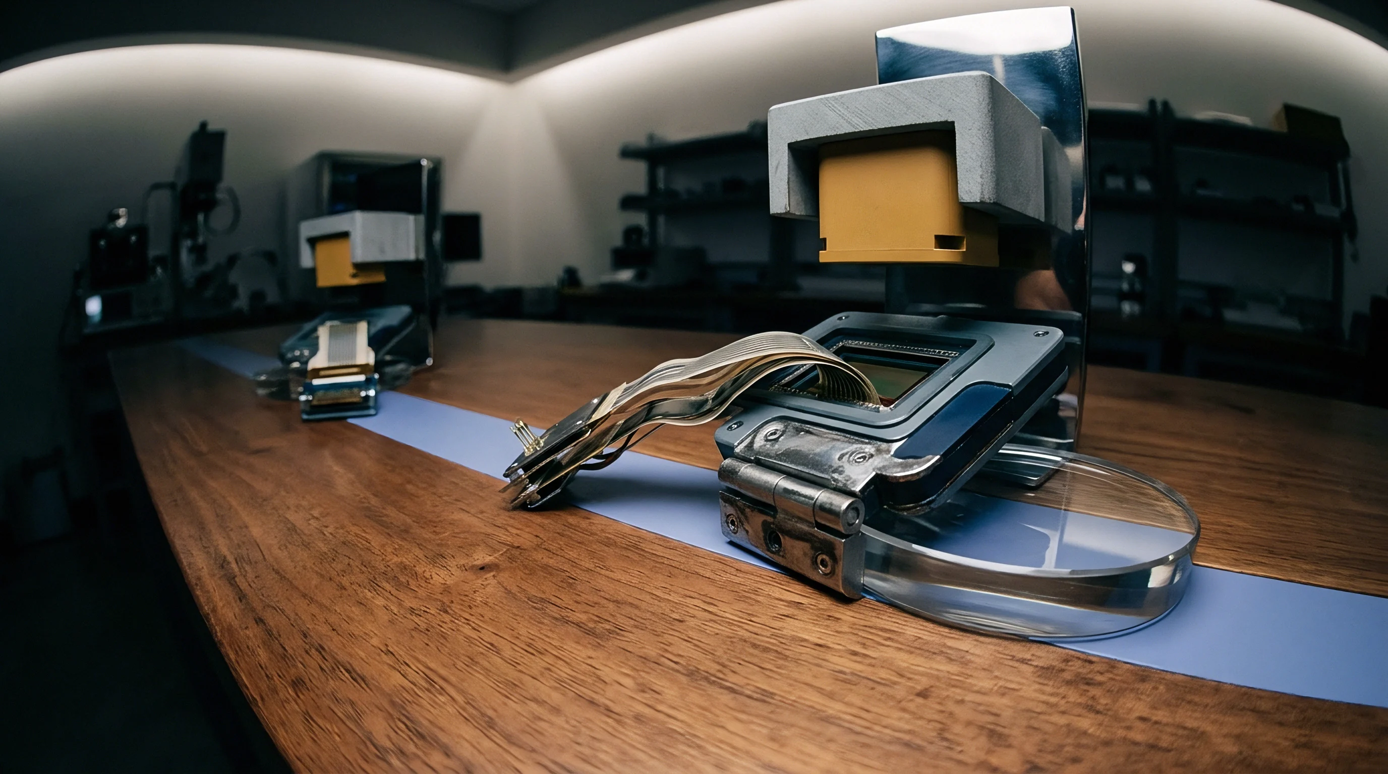
Long-term output stability separates bench-grade sensors from commercial transmitters. Silicon behaves as an elastic material with negligible mechanical hysteresis. Drift mechanisms in encapsulated silicon pressure sensors trace back to structural packaging materials, bond layers, and electrical passivations.
Creep in die-attach adhesives, relaxation of sealing glass frits, and moisture-induced surface charge accumulation on silicon dioxide dielectrics cause continuous output baseline drift under steady environmental conditions.
Die-attach materials bond the silicon chip to an intermediate header made of ceramic, Kovar, or silicon. Epoxies introduce viscoelastic creep under mechanical stress. When line pressure cycles repeatedly, polymer chains in standard conductive epoxies slip, relieving internal stress and changing zero-pressure baseline resistance.
Glass frit seals provide higher long-term dimensional stability than organic epoxies. Frit bonding requires processing temperatures near 400 degrees Celsius, which freezes in residual thermal stresses from thermal expansion mismatches between silicon and supporting headers. These locked-in stresses relax over operating life, producing monotonic drift curves.

Mechanical Relaxation in Assembly Interfaces
Drift rates follow logarithmic profiles over time, exhibiting fast changes during initial operational burn-in followed by lower rates of baseline drift. Quantifying these behaviors requires tracking performance across multi-year intervals.
- Viscoelastic Adhesive Slippage relieves assembly stresses over the first 500 hours, shifting baseline zero by 0.1 to 0.4 percent of full scale span before settling.
- Dielectric Surface Charge Trapping alters inversion layers beneath oxide passivations, drifting Wheatstone bridge balance by 0.05 percent per year under high DC excitation voltages.
- Isolation Diaphragm Work-Hardening shifts the spring rate of metallic isolation foils subjected to continuous pressure pulsation, steepening span calibration curves over millions of cycles.
- Fill Cavity Micro-Leakage through imperfect hermetic weld seams drains internal hydraulic fluid, altering volume balance and inducing catastrophic zero shifts exceeding 5 percent.
Consider a 10-bar gauge pressure transmitter deployed in an industrial setting. Baseline stability data gathered across three years reveals how different packaging configurations behave under field conditions.
| Packaging Architecture | Zero Drift (Year 1) | Zero Drift (Year 3 Cumulative) | Span Drift (Year 3 Cumulative) | Primary Mechanism |
|---|---|---|---|---|
| Parylene-Coated Die on PCB | 0.35% FSS | 0.82% FSS | 0.25% FSS | Moisture adsorption and PCB warpage |
| Gel-Potted Ceramic Header | 0.20% FSS | 0.48% FSS | 0.18% FSS | Die-attach epoxy relaxation |
| Oil-Filled 316L Welded Cell | 0.06% FSS | 0.12% FSS | 0.08% FSS | Isolation diaphragm metallurgical aging |
| Eutectic-Bonded Oil-Filled Cell | 0.03% FSS | 0.05% FSS | 0.03% FSS | Minor resistor aging in silicon bulk |
Dielectric charging represents an electronic drift path independent of mechanical packaging. DC excitation currents flowing through bridge resistors generate electric fields across surface passivation layers. Ambient moisture, ionic contaminants, or mobile sodium ions inside silicon dioxide drift toward the charged interfaces under field potentials.
This charge accumulation creates parasitical channel conductance within high-resistivity silicon substrates, changing effective bridge resistance. Pulsing sensor excitation via low-duty-cycle square waves mitigates ionic migration across the dielectric surface, halving long-term electronic drift compared to continuous DC operation.
Field recalibration plans must budget for these baseline wanderings. Specifying an annual stability figure of 0.1 percent full scale span without stating environmental conditions permits suppliers to test parts in dry, climate-controlled environments. In actual plant operations with cycling ambient temperatures and continuous vibration, real drift runs three to five times higher than clean laboratory predictions.
Failure to account for packaging relaxation forces unscheduled site interventions to re-zero field instruments that show false process wander.
Matrix
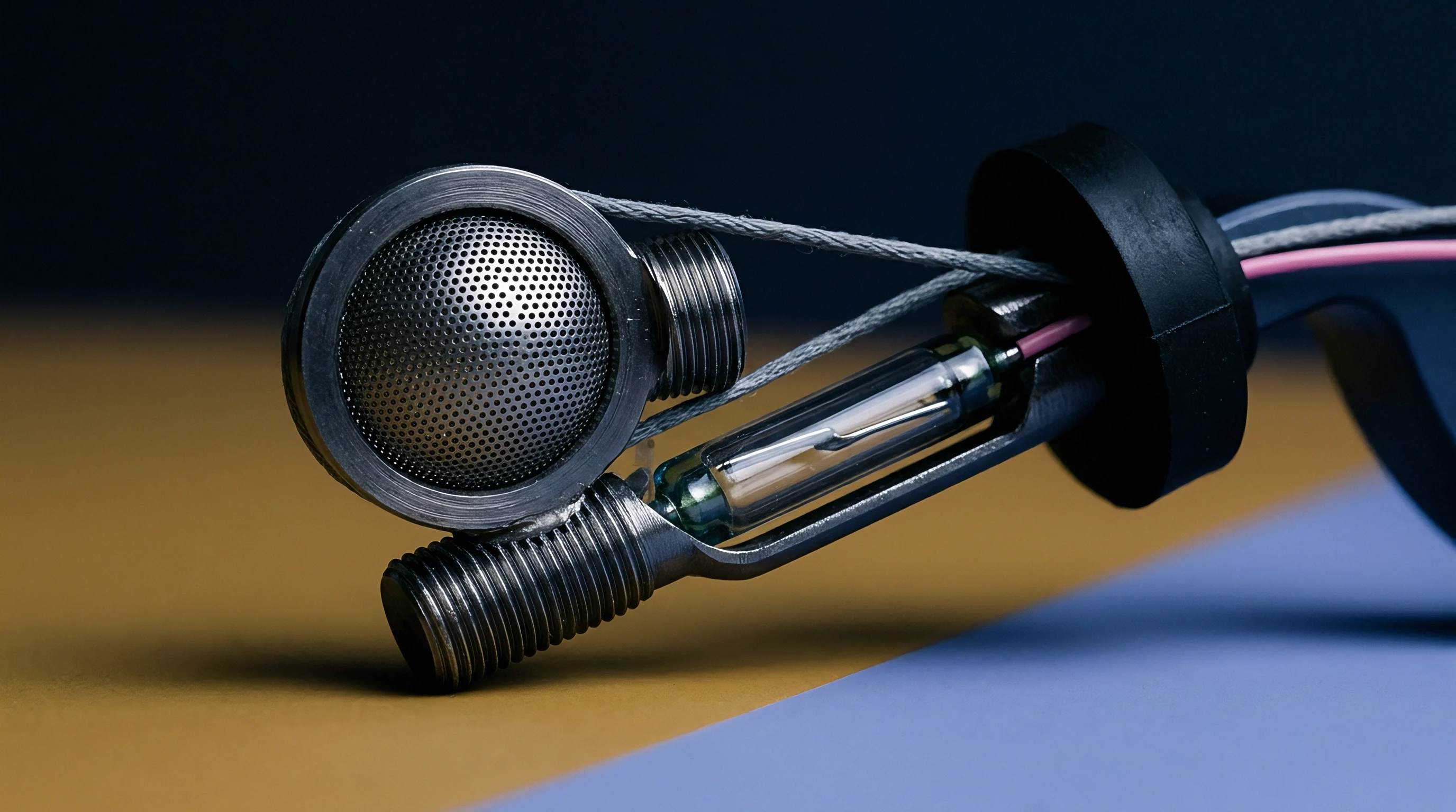
Calibrating piezoresistive silicon pressure sensors requires correcting both sensor non-linearity and temperature cross-sensitivity. Bare silicon piezoresistors exhibit a temperature coefficient of resistance between plus 15 and plus 25 percent per 100 Kelvin, accompanied by a temperature coefficient of gauge factor between minus 12 and minus 20 percent per 100 Kelvin. Pressure sensitivity drops as temperature climbs.
Compensating these thermal characteristics requires multi-dimensional mathematical calibration matrices implemented via digital signal conditioning application-specific integrated circuits.
Calibration relies on gathering real measurement nodes across pressure and temperature domains. Factory equipment places batches of sensors into automated environmental chambers coupled to digital pressure controllers. The system records raw digital counts from the primary piezoresistive bridge and an integrated temperature sensor at predetermined calibration coordinates.
These raw points form the basis for calculating individual compensation coefficients stored inside the sensor non-volatile EEPROM memory.
Mathematical Calibration Models
Calibration engines map raw bridge output and temperature readings to corrected output values using two-dimensional polynomial expansions. The order of the polynomial dictates both the achievable accuracy and the testing time required on production calibration manifolds.
Corrected pressure values follow from bivariate polynomial equations:
P_corrected = Sum over i and j of (C_ij multiplied by (S_raw minus S_zero)^i multiplied by (T_raw minus T_ref)^j)
Index i designates the pressure polynomial degree, index j designates the temperature polynomial degree, S_raw represents bridge digital counts, T_raw represents the internal temperature signal, and C_ij denotes stored factory compensation coefficients. A standard third-order pressure, second-order temperature matrix requires solving for twelve unique calibration coefficients.
A third-order bivariate calibration matrix eliminates up to 98 percent of uncompensated thermal errors across a 100-degree industrial range.
Generating coefficients for a third-order model demands minimum calibration coordinates across three temperatures: minus 20, plus 25, and plus 85 degrees Celsius, evaluated at five pressure increments: zero, 25, 50, 75, and 100 percent of full scale span. This fifteen-point matrix characterises non-linear bridge response and temperature-dependent sensitivity slope shifts. The compensation ASIC calculates corrections in real time using fixed-point arithmetic engines.
This processing holds total error bands within plus or minus 0.1 percent of full scale span across the compensated temperature envelope.
Can Two Point Factory Calibration Hold Accuracy across Full Thermal Spans?
Low-cost sensor vendors often apply two-point pressure trimming at room temperature, relying on generalized nominal compensation curves to correct for thermal shifts. This shortcut bypasses individual thermal chamber characterization to lower production testing costs. Silicon manufacturing variances yield die-to-die spreads in temperature coefficients of sensitivity of plus or minus 3 percent across a single silicon wafer.
Sensors calibrated via nominal batch curves exhibit temperature-induced span errors exceeding plus or minus 1.8 percent of full scale span when subjected to extreme operating temperatures. Maintaining error bands below 0.25 percent of full scale span across wide thermal ranges requires individual temperature-point testing for every manufactured sensor.
Automated calibration equipment must allow sufficient thermal soak times at every measurement coordinate. Rapid thermal cycling causes temperature gradients between the internal silicon element and the external reference sensor. If pressure data is captured before the encapsulated oil volume stabilizes, thermal lag corrupts the derived compensation coefficients.
A 10-bar oil-filled capsule with an internal thermal time constant of 4.5 seconds requires at least 45 seconds of soak time at each target temperature before pressure application to prevent calibration-induced hysteresis errors.
Section 6.3 of the standard equipment supply agreement governs calibration coefficient acceptance criteria, determining whether out-of-tolerance units undergo automated recalibration runs or face immediate lot rejection.


Uncertainty
Stating calibration accuracy without an accompanying uncertainty budget renders the quoted specification incomplete. A calibration certificate reporting an error of plus or minus 0.05 percent of full scale span must quantify the expanded measurement uncertainty of the calibration chain used to verify that value. International standards such as ISO/IEC 17025 and the Guide to the Expression of Uncertainty in Measurement define formal procedures for identifying, calculating, and combining all error contributors affecting a calibration procedure.
The total uncertainty of a calibrated silicon pressure sensor combines contributions from laboratory reference standards, automated test equipment, environmental variations, and intrinsic sensor limitations. Systematic errors include reference standard inaccuracies, digital multimeter resolution limits, and thermal chamber gradients. Random contributors encompass short-term bridge noise, atmospheric pressure variations in gauge calibrations, and mechanical connection stress during manifold clamping.

Derivation of a Calibration Uncertainty Budget
Building an uncertainty budget requires converting every error source into a standard uncertainty value modeled as an equivalent standard deviation. We evaluate a calibration setup for a 10-bar encapsulated transmitter tested against a deadweight piston gauge or a quartz Bourdon tube reference standard.
| Source of Uncertainty | Value (± bar) | Probability Distribution | Divisor | Standard Uncertainty (u_i) |
|---|---|---|---|---|
| Primary Reference Standard | 0.00050 | Normal (k=2) | 2.000 | 0.000250 bar |
| Reference Standard Stability Drift | 0.00020 | Rectangular | 1.732 | 0.000115 bar |
| Digital Multimeter Voltage Readout | 0.00015 | Rectangular | 1.732 | 0.000087 bar |
| Manifold Temperature Stability (±0.5°C) | 0.00040 | U-Shaped | 1.414 | 0.000283 bar |
| Barometric Variation (Gauge Reference) | 0.00010 | Rectangular | 1.732 | 0.000058 bar |
| Unit Under Test Repeatability | 0.00030 | Normal (k=1) | 1.000 | 0.000300 bar |
Standard uncertainties combine via the root-sum-square method for uncorrelated input quantities:
u_combined = Square root of (0.000250^2 + 0.000115^2 + 0.000087^2 + 0.000283^2 + 0.000058^2 + 0.000300^2)
u_combined = Square root of (0.0000000625 + 0.0000000132 + 0.0000000076 + 0.0000000801 + 0.0000000034 + 0.0000000900) = 0.000507 bar
Applying a coverage factor of k equals 2 provides an expanded uncertainty representing an approximate 95.45 percent confidence interval:
U_expanded = 2 multiplied by 0.000507 bar = 0.00101 bar (or 0.0101 percent of the 10-bar full scale span).
The Test Uncertainty Ratio evaluates whether the calibration system provides sufficient margin to certify sensor performance. If the unit under test claims a total tolerance of plus or minus 0.05 percent of full scale span (0.0050 bar), this calibration process delivers a Test Uncertainty Ratio of 0.0050 divided by 0.00101, which equals 4.95 to 1. Metrology procedures typically demand a minimum ratio of 4 to 1 to validate specification claims without complex guard-banding rules.
If the Test Uncertainty Ratio drops below 4 to 1, calibration laboratories must apply guard bands under ISO 14253-1. Guard-banding narrows acceptance criteria by subtracting the expanded uncertainty from the manufacturer tolerance limits. A sensor claiming 0.05 percent tolerance evaluated with a 2 to 1 Test Uncertainty Ratio must meet an acceptance limit of 0.025 percent during verification testing.
This tight window increases internal factory rejection rates, raising landed piece-part costs for the buyer.
Traceability chains link the working calibration standard through secondary standards to national metrology institutes such as NIST or PTB. If a vendor cannot supply calibration certificates documenting unbroken traceability chains with stated uncertainties for each step, stated accuracy claims remain unverified marketing estimates. Laboratory audits must confirm that working deadweight testers or reference controllers undergo regular recalibration cycles at accredited facilities.

Expense
Tightening sensor performance specifications steepens procurement and lifecycle costs. Sourcing engineers balance performance margins against initial unit costs, testing expenses, and field calibration intervals. Selecting an inappropriate media barrier or an unverified accuracy grade produces field failures, unexpected drift, and warranty interventions.
The base cost of a silicon pressure die represents a modest portion of total transmitter assembly expenses. Moving from a gel-potted plastic package to a welded 316L or Hastelloy capsule increases structural manufacturing costs significantly. Adding custom calibration points across extended thermal ranges raises cycle times inside expensive automated thermal chambers, directly driving up unit prices.

Cost Mechanics across Sensor Architectures
Commercial configurations exhibit distinct production and lifecycle economics across typical industrial operating lives.
- Parylene-Coated Board-Mount Elements carry unit costs between 2.50 and 6.00 dollars with room-temperature calibration, serving cost-sensitive dry pneumatic equipment that accepts 1.5 percent span errors.
- Gel-Filled Stainless Headers range from 12.00 to 22.00 dollars, utilizing three-point thermal calibration to achieve 0.5 percent accuracy across automotive cooling and engine oil systems.
- Fully Welded Oil-Filled Capsules cost between 35.00 and 75.00 dollars, requiring fifteen-point calibration matrices to achieve 0.1 percent accuracy in municipal water, hydraulics, and chemical processes.
- Corrosion-Resistant Alloy Transmitters constructed from Hastelloy C-276 exceed 140.00 dollars per unit, utilizing accredited multi-point calibration matrices for offshore oil and gas or pharmaceutical processing.
Consider an industrial automation project requiring 2,500 pressure sensing nodes across a chemical processing site. The engineering team evaluates two approaches: a standard gel-potted sensor with an annual drift of 0.4 percent of full scale span, and a hermetically sealed oil-filled sensor with an annual drift of 0.08 percent of full scale span. The site instrumentation specification mandates a maximum operating measurement tolerance of 0.5 percent of full scale span.
The standard gel-potted sensor costs 18.00 dollars per unit, requiring biannual field calibration visits to adjust for zero drift and maintain required accuracy. A qualified instrumentation technician requires 45 minutes per node, billed at an operational rate of 85.00 dollars per hour, creating an annual recalibration expense of 127.50 dollars per measurement point. Across three years of operation, ownership costs reach 400.50 dollars per sensor location.
The hermetically sealed oil-filled sensor carries an initial purchase price of 62.00 dollars. Its low baseline drift rate allows recalibration intervals to stretch out to three years while holding process tolerances. Routine field verification occurs once across the three-year period, requiring 63.75 dollars in technician time.
Total ownership costs across three years equal 125.75 dollars per measurement point. Committing higher capital expenditure during initial procurement saves the operation 274.75 dollars per location over three years, avoiding more than 686,000 dollars in field maintenance across the full facility.
A procurement specification that omits drift limits, media encapsulation chemistry, or accredited calibration requirements invites vendors to quote low-cost, inadequately isolated sensors. When these units drift out of tolerance under chemical exposure, the buyer pays for subsequent recalibration labor, warranty claims, and unscheduled plant outages.