Thermal Drift Mitigation for High Frequency FMCW Radar Transducers Installed in Narrow Vessels
High frequency FMCW radar transducers in narrow vessels mitigate thermal drift by combining low-loss thermal isolation mounts with dynamic real-time DSP phase subtraction.

Nozzle
Internal process pipes under fifty millimeters in diameter create severe wave-guiding challenges for high-frequency radar signals. Operating an 80 GHz or 120 GHz Frequency Modulated Continuous Wave (FMCW) radar transducer inside a narrow mounting neck means the beam cannot travel as if in unconfined space; it bounces off the metallic or ceramic boundary walls all the way down. Axial thermal gradients across these necks expand or contract the housing, altering interior dimensions and shifting the phase velocities of guided propagation modes.
A 50 Kelvin temperature change along a 300 millimeter stainless steel neck expands its length by roughly 0.25 millimeters and shifts the internal diameter enough to move the cutoff frequencies of high-order TE and TM modes. For narrow vessel level measurements where full-scale target travel may be under two meters, uncorrected millimeter-scale expansions distort measurement accuracy.
Narrow vessel geometries concentrate microwave energy into a tight channel. At W-band (75 GHz to 110 GHz) and D-band (110 GHz to 170 GHz), high-frequency radar wavelengths run between 1.75 millimeters and 4.0 millimeters. Because these wavelengths fall right on the scale of internal weld seams, surface roughness, and machining tolerances, local thermal expansion alters the relative phase of internal reflections.
The result is fixed-distance false targets ~ nozzle clutter or antenna ringing. As ambient or process temperatures cycle, this false reflection shifts in phase relative to the true liquid interface echo. The receiver mixer’s beat frequency shifts with it, driving an apparent level drift even while the actual liquid height never moves.
Standpipe Geometries and near Field Propagation Traps
Internal welds, threaded joints, or diameter steps in process connection necks trigger strong ringing. In narrow vessels, nozzle length often exceeds inner diameter by more than five to one. At these ratios, the radar horn or planar lens antenna works deep inside its reactive near-field region relative to the pipe walls.
The radiated field grazes internal surfaces at shallow angles, building a complex interference pattern of coaxially guided modes. As heat climbs from hot vessel vapors into the mounting flange, an axial thermal gradient drives uneven radial pipe expansion, keeping the upper flange near ambient temperature while the lower connection hits process temperature.
This uneven expansion warps the pipe’s cross-sectional roundness, splitting circular TE11 modes into elliptical modes with divided polarization vectors. Because the receiver antenna array is tuned for a single linear polarization, the primary signal channel loses amplitude and suffers phase retardation. A 3-millimeter ovality caused by asymmetric thermal clamping across a 40-millimeter nozzle shifts the primary reflection centroid by up to 3.8 millimeters in apparent distance ~ completely independent of any drift inside the semiconductor transceiver chip itself.
An uncompensated thermal shift of 15 Kelvin in an 80 GHz MMIC junction alters the beat frequency by 24 kilohertz, shifting the perceived ullage reading by 4.5 millimeters at a 2-meter target distance.
Vessels with internal agitation, boiling liquids, or thermal jackets push transient heat up into the mounting neck through convection and conduction. Convective thermal plumes moving through a stilling well cause localized density variations in the vapor space, causing the dielectric constant to fluctuate according to the Clausius-Mossotti relationship. While the refractive index shift in atmospheric air is negligible, narrow vessels carrying heavy hydrocarbon vapors, volatile solvents, or pressurized steam experience pronounced velocity shifts.
FMCW radar distance calculations rely directly on the speed of light through the medium in the neck. If localized vapor temperature drops by 80 Kelvin down the length of the standpipe, phase velocity speeds up, leading the radar to report a fluid level closer to the sensor than it actually is.
Process Window Thermal Gradients and Permittivity Drift
Solid isolation discs positioned between transmitter and vessel atmosphere develop radial heat gradients. High-pressure narrow vessels rely on physical process barriers made of Polytetrafluoroethylene (PTFE), Polyether ether ketone (PEEK), Fused Silica, or Synthetic Sapphire to isolate delicate millimeter-wave electronics from corrosive process media, high pressures, and extreme heat. But the dielectric constant of these polymers and ceramics drifts with temperature.
The real part of the relative permittivity ( εr ) sets both the refractive index and the phase delay of the microwave signal traversing the window disc.
As process temperatures rise, the center of the isolation window warms faster than its clamped outer edge. This radial temperature gradient builds a non-uniform refractive index profile across the lens face, producing a thermal lensing effect that focuses or defocuses the microwave beam based on the sign of the material’s temperature coefficient of permittivity ( dεr / dT ). PTFE undergoes a sharp step-change in density and dielectric constant around its 19 °C phase transition, ruling it out for precision narrow-vessel windows unless active thermal modeling is used.
Fused Silica offers excellent thermal stability with an expansion coefficient near 0.5 × 10⁻⁶ , K-1 , though high manufacturing costs restrict its broader use in commercial process instruments.
Physical failure modes in narrow vessel radar installations stem from structural expansion, material phase transitions, and density shifts in the vapor medium:
- Structural neck elongation shifts the mechanical zero-reference point of the antenna flange relative to the vessel’s bottom datum point.
- Radial thermal distortion warps the internal cross-section of narrow standpipes, triggering higher-order mode conversions that distort the primary return spectrum.
- Dielectric window phase shift changes the electrical path length through the pressure seal, creating an apparent distance offset proportional to lens thickness.
- Vapor phase refractive index drift changes propagation speed inside the confined neck space, corrupting time-of-flight beat frequency calculations.
- Thermal clutter migration shifts the phase and amplitude of fixed nozzle reflections, causing false spectral peaks to obscure the true liquid interface signal.
Choosing window materials requires balancing dielectric loss, mechanical strength, and thermal drift behavior. Table 1 outlines the physical and electromagnetic properties of common window materials tested across standard process temperature ranges.
| Material Grade | Thermal Expansion Coefficient (10-6 , K-1) | Dielectric Constant εr (at 80 GHz) | Temperature Coefficient dεr/dT (10-4 , K-1) | Loss Tangent tan δ (at 80 GHz) | Max Continuous Temperature (°C) |
|---|---|---|---|---|---|
| Standard PTFE | 120.0 | 2.05 | -4.10 | 0.0004 | 260 |
| Modified PTFE (TFM) | 100.0 | 2.04 | -2.80 | 0.0003 | 260 |
| PEEK (Unfilled) | 45.0 | 3.12 | +1.20 | 0.0031 | 250 |
| Fused Silica (99.99%) | 0.5 | 3.81 | +0.15 | 0.0001 | 1100 |
| Synthetic Sapphire | 5.3 | 9.30 | +0.80 | 0.0001 | 1700 |
| Data measured across -40 °C to +200 °C operating window using split-post dielectric resonator techniques at 80 GHz baseline. | |||||
Ignoring physical expansion and dielectric phase shifts in narrow vessel nozzles produces systematic measurement errors. An uncorrected 3-millimeter elongation of the mounting neck alongside a 2-millimeter dielectric path stretch shows up as a 5-millimeter error in reported level. In applications like pharmaceutical dosing tanks or chemical metering columns, a 5-millimeter ullage error wipes out the entire allowable tolerance window, setting off false high-level alarms or driving costly overfills.

Silicon
Transceiver integrated circuits operating at 79 gigahertz turn minor semiconductor junction shifts into range measurement errors. Modern FMCW radar systems use integrated Silicon-Germanium (SiGe) BiCMOS or complementary metal-oxide-semiconductor (RF-CMOS) monolithic microwave integrated circuits (MMICs). These single-chip transceivers combine the voltage-controlled oscillator (VCO), fractional-N phase-locked loop (PLL), power amplifier (PA), low-noise amplifier (LNA), quadrature mixers, and baseband programmable gain amplifiers.
Inside an industrial enclosure, the silicon die experiences junction temperatures from -40 °C to above +125 °C, heated both externally by vessel connections and internally by power dissipated in the PA and digital core.
An FMCW radar chip’s operating frequency is controlled by the instantaneous voltage fed to its internal VCO. In an ideal setup, the ramp generator creates a linear frequency sweep over time, defined by the chirp slope γ = B / Tc , where B is the sweep bandwidth (typically 4 GHz in the 77 ~ 81 GHz band) and Tc is chirp duration. The radar mixer down-converts received reflections against the instantaneous transmit signal, generating an intermediate frequency (IF) beat tone fb.
This beat frequency maps directly to target distance R via fb = (2 · R · γ) / c , where c is the speed of light. Any thermal fluctuation that skews the chirp slope γ corrupts distance reading R.
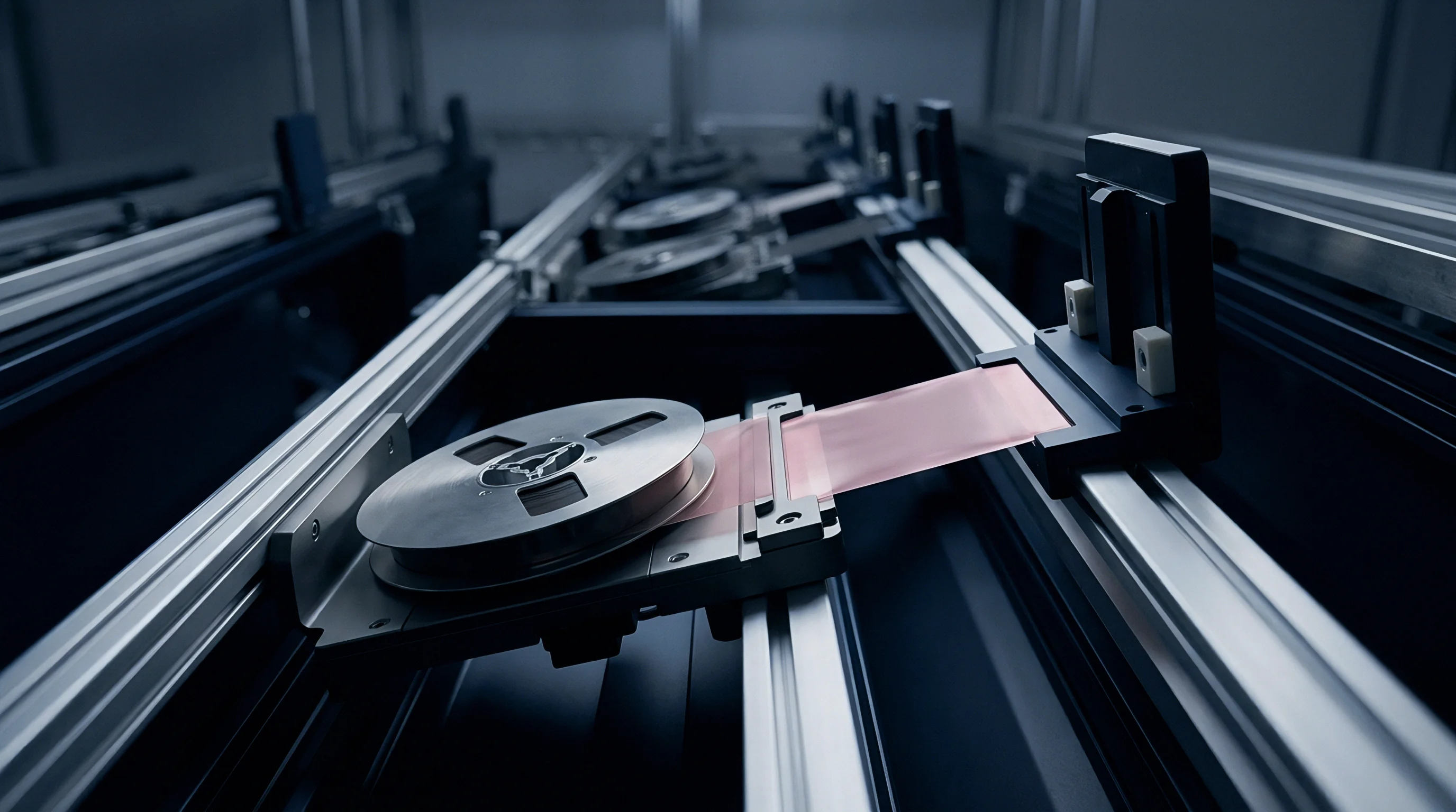
Voltage Controlled Oscillator Chirp Slope Variation over Junction Temperature
Maintaining a linear sweep requires uniform tuning steps across the full modulation bandwidth. Silicon transceivers control VCO frequency using on-chip varactor diodes, whose capacitance varies non-linearly with both tuning voltage and semiconductor junction temperature Tj. As die temperature rises, the built-in potential of the varactor PN junctions shifts by about -2 millivolts per degree Celsius.
This movement alters the VCO’s frequency-versus-voltage response, bending what should be a straight frequency ramp.
If chirp slope γ(t) drifts during the sweep, beat frequency fb loses its pure sinusoidal tone. The signal spreads across adjacent frequency bins in the Fast Fourier Transform (FFT) spectrum ~ a condition known as spectral broadening or chirp non-linearity error that degrades spatial resolution. In narrow vessels, this spreading lets the powerful reflection from the nozzle flange bleed into neighboring bins, masking weak echoes from liquid interfaces near the pipe outlet.
Temperature spikes inside the MMIC degrade phase noise as well. Thermal noise in the VCO resonant tank tracks absolute temperature in Kelvin, lifting the single-sideband phase noise floor. A 50 Kelvin jump in junction temperature usually degrades phase noise at 1 MHz offset from the carrier by 3 to 5 dBc/Hz. This elevated phase noise lowers the signal-to-noise ratio (SNR) of the intermediate frequency signal, driving up measurement jitter and complicating detection of low-permittivity fluids like hydrocarbons or liquefied gases in narrow standpipes.
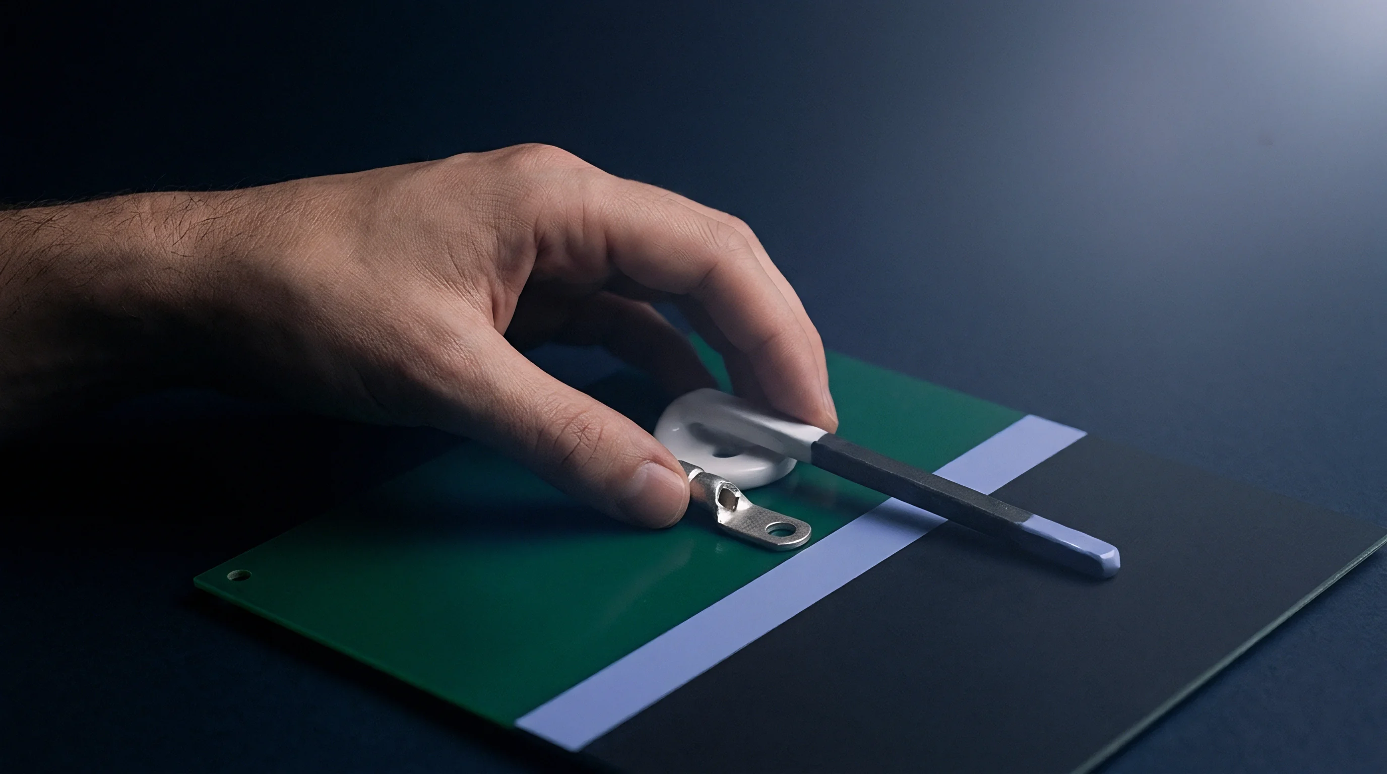
Monolithic Array Substrate Expansion and Antenna Phase Center Displacement
Microstrip patch elements etched onto high-frequency laminates shift electrical length as heat builds up. Modern 80 GHz transducers often integrate planar patch antenna arrays directly onto organic or ceramic substrates like Rogers RO3003 or Megtron 6. These materials exhibit distinct thermal coefficients of dielectric constant ( dεr / dT ) and linear coefficients of thermal expansion (CTE along X, Y, and Z axes).
When the package heats, physical patch dimensions expand while substrate dielectric constant drops.
A patch antenna’s physical length sets its resonant frequency and phase response. Substrate expansion alters spacing between array elements, distorting the phase relationship across the antenna face. This misalignment moves the antenna phase center ~ the apparent origin point of the electromagnetic wave.
In narrow vessel geometry, a 0.5-millimeter shift in phase center shows up directly as a 0.5-millimeter error in reported ullage. At the same time, phase center displacement widens the primary beam and raises side-lobe levels, directing more energy into the metallic walls of narrow nozzles and compounding near-field clutter.
Table 2 outlines the thermal behavior and sensitivity of key internal MMIC functional blocks to junction temperature shifts.
| MMIC Circuit Block | Primary Physical Parameter | Nominal Value (at 25 °C) | Thermal Coefficient | Impact on Radar Output |
|---|---|---|---|---|
| VCO Varactor Core | Tuning Sensitivity (Kvco) | 1.2 GHz/V | +1.8 MHz/V/°C | Chirp non-linearity and range bin spreading |
| Fractional-N Charge Pump | Current Mismatch (Icp) | 500 µA | +0.45 µA/°C | Fractional spur elevation and phase noise degradation |
| Power Amplifier (PA) | Saturated Output Power (Psat) | +13 dBm | -0.035 dB/°C | Loss of dynamic range at high operating temperatures |
| Low Noise Amplifier (LNA) | Noise Figure (NF) | 8.5 dB | +0.022 dB/°C | Reduced signal-to-noise ratio for distant fluid targets |
| On-Chip Delay Line | Group Delay (τref) | 1.25 ns | +0.12 ps/°C | Zero-distance baseline drift in internal calibration loops |
Chip vendors routinely market high-frequency radar ICs with internal digital temperature sensors as having built-in drift compensation. Placing a single sensor on the digital corner of the die fails to capture local junction temperatures in the power amplifier or VCO core, which can run 20 Kelvin hotter than neighboring silicon during active chirping. Built-in lookup tables can control thermal drift within specification, provided the package baseplate temperature stays within a strict 10 Kelvin range.
That qualifier passes the thermal management problem straight back to mechanical designers, since holding an industrial enclosure to such tight limits inside a hot plant is nearly impossible without heavy-duty thermal mounting hardware.
Mount
Mechanical isolation fittings keep delicate mmWave electronics safe from high-temperature process flanges. Processing vessels in chemical plants, refineries, and power generation often operate above +200 °C, whereas commercial radar electronics typically cap maximum PCB temperatures at +85 °C. Bridging that thermal gap requires dedicated mounting standoffs, conductive heat breaks, and carefully planned mechanical interfaces. The goal is to insert high thermal resistance along the conductive path while keeping the assembly rigid and microwave losses low.
Conductive heat transfer follows Fourier’s Law, Q = -k · A · (dT / dx) , where Q is heat flow rate, k is material thermal conductivity, A is cross-sectional area, and dT / dx is the thermal gradient along the axis. Minimizing Q means paring back metal cross-section, lengthening path x , or choosing materials with low thermal conductivity. Standard 316L stainless steel has a thermal conductivity of roughly 16 , W/(m·K).
Specialized isolation necks turn to Hastelloy C-276 ( k ≈ 10 , W/(m·K) ) or titanium alloys like Ti-6Al-4V ( k ≈ 6.7 , W/(m·K) ) to choke off conductive heat flowing from the process flange toward the radar housing.
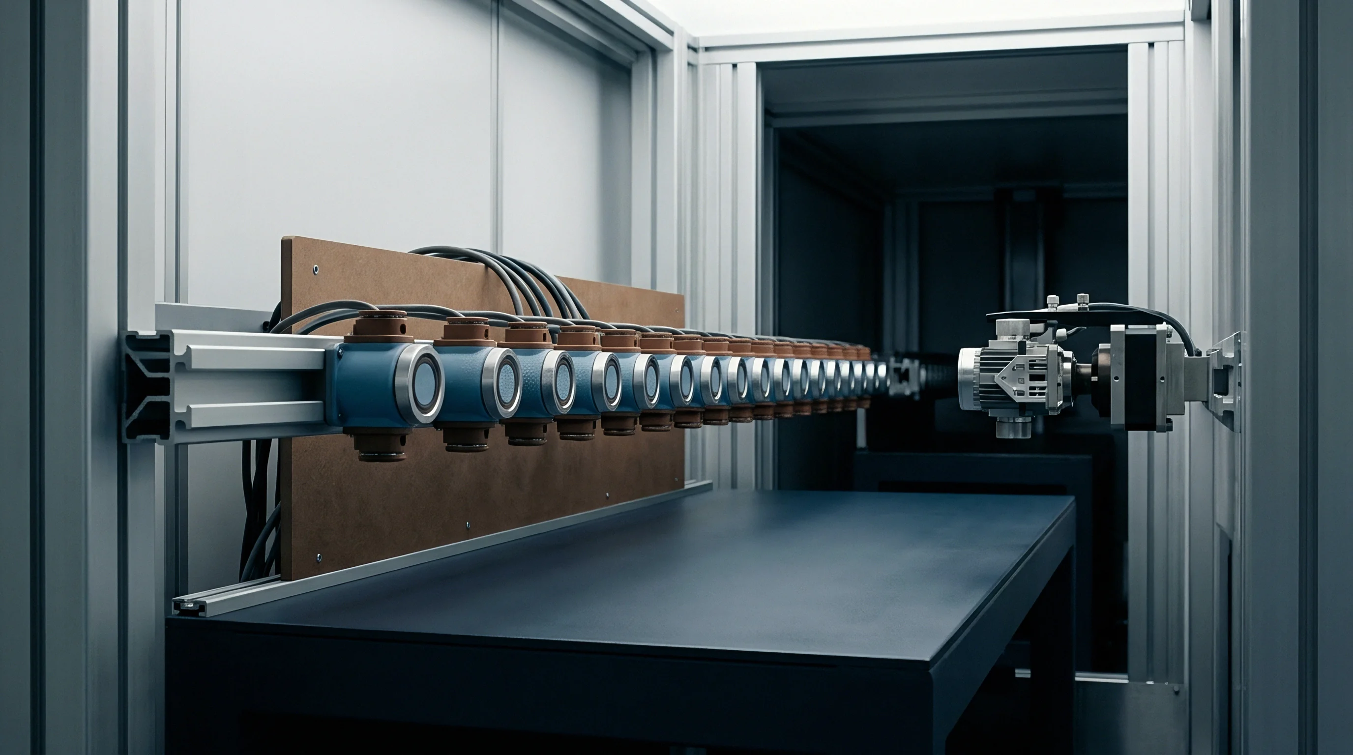
Conductive Isolation Structures and Materials Selection
Inserting waveguide extensions between antenna horn and housing provides effective thermal isolation. A hollow waveguide wall has a tiny conductive cross-section compared to a solid flange, dramatically dropping heat transfer. Uninsulated waveguide sections, however, form internal air columns prone to convection currents and moisture condensation.
Filling the interior with low-loss dielectric rods ~ like fused silica or low-density expanded PTFE ~ blocks internal convection while preserving a sealed path for mmWave transmission.
Cooling fins on the exterior neck boost radiative and convective heat exchange with surrounding air. Under natural convection, finned necks lower internal waveguide transition temperatures by up to 100 Kelvin over a 150 millimeters axial span. When ambient air is stagnant or reaches +60 °C inside protective sunshades, natural convection degrades.
In those cases, passive finned mounts must be oversized or paired with ceramic thermal breaks like Zirconia ( ZrO2 ), which offers high compressive strength alongside very low thermal conductivity ( k ≈ 2.0 , W/(m·K) ).
Systematic selection of thermal isolation standoff components requires evaluating mechanical, thermal, and microwave criteria:
- Audit process temperature limits to establish the maximum continuous temperature differential ( Δ T ) between the process flange and the radar enclosure.
- Calculate conductive heat flux through candidate mounting geometries to verify that total heat flow does not exceed the cooling capacity of the enclosure heatsink.
- Verify structural resonance frequencies of extended isolation necks under plant vibration profiles to prevent mechanical fatigue failure of internal mmWave interconnects.
- Evaluate microwave insertion loss across the operating frequency band for all internal dielectric seals and waveguide heat-break interfaces.
- Inspect mechanical expansion matching between dissimilar metals and ceramics in the assembly to prevent seal degradation during rapid thermal cycling.
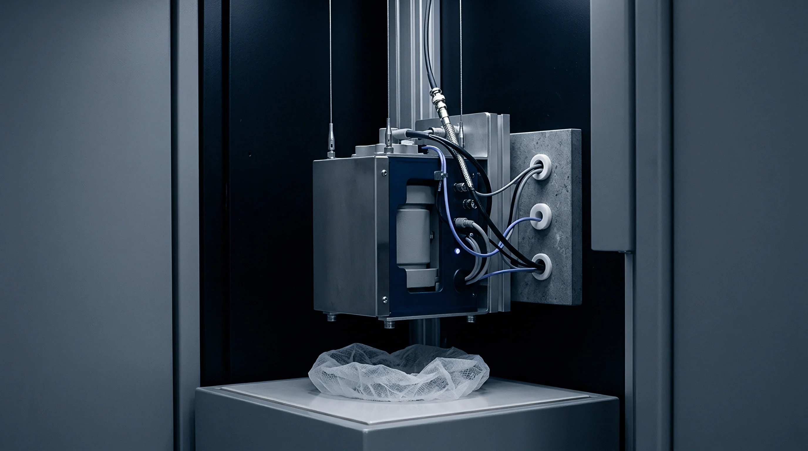
Active Thermoelectric Stabilization against Ambient Transients
Peltier modules keep substrate temperatures stable during fast ambient swings. Passive cooling handles steady process heat, but it cannot stop temperature shifts driven by day-night cycles, direct sun, or weather events. Direct sunlight on an unshielded aluminum housing can drive internal temperatures up 30 Kelvin in 20 minutes ~ creating dynamic drift that standard calibration loops cannot keep up with.
Active thermal management mounts Thermoelectric Coolers (TECs) directly behind the high-frequency radar MMIC. A closed-loop PID controller tracks a thermistor embedded in the MMIC heat-slug, modulating Peltier current to hold the chip substrate steady at +45 °C despite changing ambient conditions. This active control stops VCO chirp drift and phase center movement at the source.
But TECs draw 2 to 5 Watts of continuous power, ruling them out for two-wire 4-to-20mA loop-powered instruments, which must rely on passive isolation paired with digital compensation algorithms.
Evaluating trade-offs between physical standoff structures involves comparing material costs, thermal attenuation rates, and RF losses across standard high-frequency mounting configurations, as summarized in Table 3.
| Mounting Architecture | Materials Used | Thermal Resistance Rth (K/W) | RF Insertion Loss at 80 GHz (dB) | Max Process Temp (°C) | Added Mechanical Length (mm) |
|---|---|---|---|---|---|
| Standard Solid Flange | 316L Stainless Steel | 2.5 | 0.1 | 120 | 0 |
| Finned Metal Neck | 316L Stainless Steel | 14.8 | 0.3 | 200 | 150 |
| Hastelloy Choke Neck | Hastelloy C-276 | 28.4 | 0.4 | 250 | 150 |
| Ceramic Waveguide Break | Zirconia / Fused Silica | 65.0 | 1.2 | 400 | 100 |
| Active TEC Module Enclosure | Anodized Al / Bismuth Telluride | Active Control | 0.2 | 150 | 50 |
Commercial contracts for process instrumentation frequently mandate strict compliance with environmental protection standards. According to Clause 5.2 of IEC 61298-2, process control devices subjected to thermal step changes must demonstrate that ambient temperature effects do not induce span errors exceeding the manufacturer’s declared accuracy class across the full operational temperature envelope.
Chirp
Phase-locked loop sweeps must stay strictly linear across the modulation spectrum to avoid range blurring. When physical isolation and semiconductor thermal controls fall short of eliminating thermal shifts, DSP routines in the radar microcontroller compensate for residual drift. High-frequency FMCW radars digitize the intermediate frequency (IF) beat signal using high-resolution ADCs sampling at up to 50 Megasamples per second, then run Fast Fourier Transforms (FFTs) to generate a complex distance spectrum.
Thermal drift distorts phase and amplitude across spectral peaks in the distance spectrum. If thermal gain drops in the VCO circuit shrink sweep bandwidth B , range resolution cell size ~ defined as Δ R = c / (2 · B) ~ widens. An 80 GHz radar with a nominal 4 GHz sweep bandwidth achieves 37.5 millimeters theoretical range resolution.
If heat shrinks that bandwidth to 3.6 GHz, resolution degrades to 41.6 millimeters, causing adjacent reflections (such as a liquid meniscus right near a nozzle lip) to blur into a single peak.

How Does Internal Phase Tracking Eliminate Chirp Error?
Secondary internal loops measure transmit waveform phase before it reaches the antenna horn. For real-time tracking, precision FMCW transceivers incorporate an internal calibration path ~ a high-Q transmission line or delay structure built directly onto the substrate. A directional coupler taps off a fraction of transmit MMIC power, routes it through this fixed delay line, and mixes it with the local oscillator to generate a reference beat frequency fref.
Because internal delay line length is fixed, any drift or phase movement in reference beat frequency fref comes entirely from thermal drift inside the synthesizer, VCO, or mixing stages. The DSP evaluates the phase of fref at the start of every chirp. Comparing observed reference phase against factory-calibrated baseline phase yields a phase correction vector, which is subtracted from the primary target FFT on a chirp-by-chirp basis ~ canceling electronic thermal drift before distance calculation algorithms execute.
Executing an internal delay-line baseline compensation sequence requires a structured execution flow inside the radar firmware loop:
- Initiate the FMCW frequency sweep cycle across the 77 ~ 81 GHz carrier band.
- Sample the reference IF beat signal generated by the internal calibration path using a secondary ADC channel.
- Compute the Fast Fourier Transform of the reference IF signal to extract instantaneous phase and peak bin frequency.
- Compare the calculated reference peak position against the non-volatile memory baseline value logged during factory calibration at 25 °C.
- Generate a phase correction matrix and apply it to the main receiver measurement channel data before running primary target detection algorithms.

Dynamic Baseline Subtraction and Spectral Centroid Compensation
Reflections from fixed internal structures shift frequency bins as housing temperatures change. In narrow vessels, background clutter from nozzle steps, internal welds, and rungs dominates the baseline spectrum. When transducer temperature shifts, clutter phase rotates relative to the liquid reflection.
Static background subtraction ~ subtracting a clutter profile recorded during commissioning ~ fails during thermal swings because the live profile moves away from the stored baseline.
Advanced DSP engines use dynamic baseline clutter tracking to handle this. The algorithm continuously tracks phase and amplitude on known fixed clutter peaks, such as nozzle flange echoes. As housing temperatures shift, the DSP updates complex coefficients in the clutter map in real time, moving the baseline spectrum along with measured temperature.
This dynamic subtraction pulls out the true liquid reflection even when it sits 20 dB below surrounding clutter echoes.
Clause 6.3 of IEC 60770-1 dictates that span error evaluation must include the full thermal transition envelope rather than static equilibrium temperature points.
With clutter cleared, the DSP pinpoints the center of the liquid reflection peak. Standard FFT math limits distance resolution to discrete bin centers; sub-millimeter precision requires spectral centroid interpolation, fitting a polynomial or Gaussian curve across the peak bin and its neighbors. Rising thermal noise distorts peak symmetry and skews interpolation, but adaptive windowing functions (like Kaiser-Bessel windowing with a thermally scaled beta parameter) restore peak symmetry across operating temperatures.
Despite advanced real-time digital phase tracking and dynamic clutter mapping, a fundamental processing question remains open: can firmware algorithms reliably distinguish between a rapid apparent level shift caused by a thermal shock event on a narrow metallic nozzle and a true rapid fluid level drop caused by emergency vessel pump-out?


Chamber
Environmental test chambers simulate thermal cycles to verify measurement stability. Bench testing high-frequency FMCW transducers requires specialized chambers fitted with microwave-transparent windows or internal mmWave absorbers. Simply placing an electronic module inside a standard oven does not work for narrow-vessel radar; the antenna array and process window must see simulated fluid and nozzle gradients while the housing undergoes ambient temperature swings.
A rigorous verification bench mounts the transducer on a 50-millimeter test pipe inside a climate-controlled chamber, aiming at an external microwave reflector on an optical rail. The chamber ramps ambient air from -40 °C to +85 °C at controlled rates (such as 1 Kelvin per minute and 5 Kelvin per minute) while a liquid loop heats the mounting flange up to +200 °C. Laser interferometers accurate to better than 0.01 millimeters track true physical distance to provide ground-truth reference data.
Environmental Profile Characterization and Temperature Step Protocol
Ramping ambient temperature at controlled rates exposes thermal hysteresis in mmWave packaging. Hysteresis shows up when a transducer reports different distance readings at the same temperature depending on whether it arrived there while heating or cooling. Stress relaxation in plastic lenses, thermal lag between the silicon die and housing thermistor, and mechanical creep in solder joints all drive these hysteresis loops.
Testing protocols hold the transducer at discrete soak steps (-40 °C, -20 °C, 0 °C, +25 °C, +50 °C, +85 °C) for at least two hours each to reach thermal equilibrium. Drift measured during transitions reveals the dynamic thermal response coefficient ( mm/K/min ), showing how sharply sudden ambient swings degrade accuracy before digital compensation catches up.
Thermal compensation algorithms fail when internal temperature sensors measure PCB copper temperatures instead of the semiconductor junction temperature itself.

Error Budget Decomposition across Temperature Limits
Combining individual drift mechanisms establishes an overall error boundary for distance readings. Test engineers build thermal error budgets that aggregate physical and electronic drift across the operating range. Root-sum-square summation gives a realistic estimate of total measurement uncertainty, assuming individual error sources are uncorrelated.
Table 4 illustrates a complete worked thermal error budget for an 80 GHz FMCW radar transducer operating on a 50-millimeter inner diameter by 200-millimeter long narrow stainless steel nozzle across a -40 °C to +85 °C ambient range with process flange heat at +150 °C.
| Drift Mechanism Source | Physical Root Cause | Uncompensated Error (mm) | Compensation Method Applied | Residual Error (mm) |
|---|---|---|---|---|
| MMIC Synthesizer Chirp Drift | VCO varactor thermal nonlinearity | ± 4.20 | Internal delay-line phase loop | ± 0.25 |
| Nozzle Metallic Expansion | Stainless steel axial growth | ± 0.48 | Flange temperature model lookup | ± 0.05 |
| Dielectric Window Phase Delay | PEEK lens dεr/dT shift | ± 1.15 | Multi-point factory temp matrix | ± 0.12 |
| Antenna Phase Center Shift | Substrate dimensional CTE growth | ± 0.35 | Fixed offset subtraction in DSP | ± 0.08 |
| Nozzle Near-Field Clutter Shift | Elliptical mode phase alteration | ± 2.80 | Dynamic baseline subtraction | ± 0.30 |
| Vapor Density Permittivity Shift | Vapor refractive index drop | ± 0.60 | External process temp input | ± 0.10 |
| Root-Sum-Square Total Error | Combined operational drift | ± 5.23 | Full Hardware & DSP Mitigation | ± 0.43 |
Soaking the transducer at thermal equilibrium for several hours remains the only reliable technique for separating transient mechanical expansion stress from true semiconductor electrical drift.

Contract
Procurement specs set strict limits on distance drift over operating temperature ranges. Buying high-frequency FMCW radar transmitters for narrow vessels in chemical or pharmaceutical plants requires clear performance guarantees against uncompensated drift. Commercial datasheets routinely feature headlines like “±1 millimeter accuracy” without making clear that the figure applies only at 20 °C room ambient with no process flange heat load.
In narrow vessel service, actual accuracy of an uncompensated instrument often degrades to ±5 millimeters or worse under process heat and solar exposure. To prevent disputes after installation, procurement engineers write explicit thermal drift limits into the Request for Quotation (RFQ) and purchase specifications. The spec must define maximum allowable error across the full operating envelope: ambient temperature (-40 °C to +85 °C), process flange temperature (-40 °C to +200 °C), and maximum process ramp rate (such as 10 Kelvin per minute).
Specification Dossiers and Thermal Performance Warranties
Datasheet accuracy numbers measured at room temperature hide significant operational drift. Specifications for precision level instruments should require vendors to supply certified factory calibration records for every unit delivered. Factory profiling cycles each completed assembly in an automated chamber across its operating range, logging raw and compensated distance against an optical laser reference standard.
A binding procurement clause for narrow-vessel radar instruments specifies clear verification conditions prior to shipment acceptance:
- Full-envelope temperature verification requires suppliers to demonstrate declared accuracy across the entire ambient and process temperature envelope, rather than relying on room-temperature mathematical models.
- Thermal step response bounds require that after a 30 Kelvin step change in flange temperature, the instrument returns to within 0.1% of full-scale accuracy within 15 minutes.
- Nozzle clutter stability criteria require vendors to guarantee that clutter suppression functions without manual re-mapping over the full operating temperature range.
- Individual unit factory calibration curves must be programmed into non-volatile EEPROM memory on the instrument, accompanied by a digital test certificate signed by quality management.
Commercial Terms for Factory Calibrated Thermal Compensation Curves
Factory thermal cycling adds manufacturing cost but guarantees field precision. Achieving sub-millimeter level stability across temperature extremes requires individual thermal calibration. High-volume commercial radars usually rely on batch-typical compensation, flashing a curve derived from ten prototype units into thousands of production sensors.
Because silicon die variation, packaging tolerances, and lens clamping forces vary unit to unit, batch compensation leaves residual thermal errors up to ±3 millimeters.
Individual multi-point calibration requires soaking each production unit at five or more temperatures in a chamber and writing custom correction coefficients directly to internal DSP flash. This testing adds 45 to 90 minutes per unit and increases landed cost by 15% to 25%. In narrow vessels where process tolerances are tight and media values high, that upfront cost is negligible compared to the expense of process upsets, off-spec batches, or safety trips caused by measurement drift.
Purchase agreements can specify terms requiring vendors to replace units and cover field re-calibration labor if an installed sensor drifts beyond contract limits within the first 24 months of operation. Holding suppliers accountable with explicit warranty liabilities ensures vendor engineering teams thoroughly analyze nozzle geometries, standoff designs, and dielectric window profiles before delivering hardware to the site.