State Augmented Kalman Filter Synthesis for Nonlinear Viscoelastic Sensor Assemblies
Augmenting Kalman filter state vectors with Maxwell relaxation variables eliminates viscoelastic drift in polymer-packaged sensor assemblies.


Rheology
Silicon strain gauge elements bonded with structural polyurethane exhibit measurable time-dependent displacement decay under step strain inputs at 25 degrees Celsius. When mechanical transducers incorporate polymeric substrates, elastomeric isolators, or structural adhesives, material deformation deviates from linear elasticity. Polymers deform elastically while flowing viscously at the same time, producing time-dependent stress relaxation, mechanical hysteresis under dynamic cycling, and baseline offset drift under sustained preloads, with stress decay following exponential paths.
Standard state estimators that treat sensor bodies as pure springs run into systematic prediction errors because unmodeled viscoelastic force components distort the filter innovations sequence.
Modeling these effects starts with the Boltzmann superposition principle, which assumes that the strain response to a complex stress history is the sum of responses from each individual stress increment. In physical assemblies subjected to strains exceeding 0.5 percent, however, material behavior becomes nonlinearly viscoelastic. Tensile modulus starts depending on strain, and relaxation rates accelerate at higher deformations.
Lumped mechanical models represent this behavior through networks of elastic springs with specific stiffness constants and viscous dashpots with damping coefficients.
Polyurethane sensor potting compounds exhibit a 14 percent stress relaxation drop over 100 hours at 23 degrees Celsius under a constant 1.0 percent shear strain.
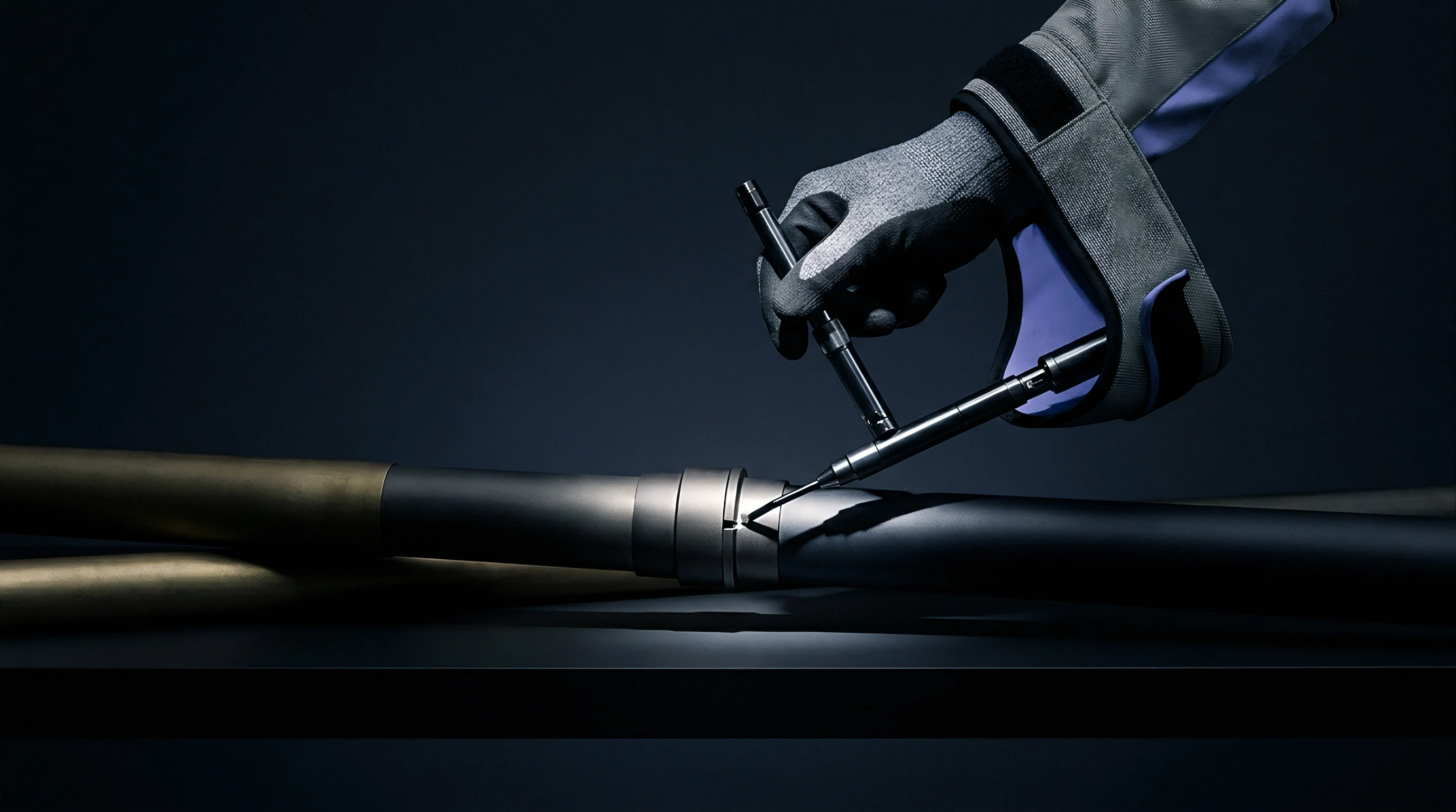
Viscoelastic Mechanics in Sensor Enclosures
Structural polymers used for transducer encapsulation store mechanical energy through internal molecular rearrangements. Under initial deformation, polymer chains stretch elastically. Over longer periods under constant displacement, these long-chain molecules slip past one another, dissipating stored strain energy as heat and corrupting low-frequency readings.
As a result, the measured output of a force transducer mounted on a viscoelastic dampening pad drops over time while the external load stays static.
Accounting for these errors requires isolating the specific physical mechanisms introduced by polymer packaging elements.
- Creep Induced Offset Drift ~ Static force measurements decay over extended loading cycles as molecules slowly realign inside the polymer matrix.
- Hysteresis Loop Widening ~ Cyclic dynamic loading introduces phase lags between applied excitation and sensed output, broadening the force-strain envelope.
- Thermal Relaxation Acceleration ~ Temperature spikes shorten internal polymer relaxation time constants according to empirical shift factor equations.
- Modulus Nonlinearity ~ Mechanical stiffness drops sharply once applied strain exceeds the assembly’s linear viscoelastic threshold.
Relaxation time constants span several orders of magnitude, from milliseconds for local chain segment movement to several days for bulk molecular entanglements. Simple low-pass filtering cannot correct these material dynamics because mechanical strain memory depends directly on loading history. Stripping out low-frequency offset shifts removes true physical motion along with viscoelastic creep.
An effective estimator instead incorporates internal material states that mirror the relaxation dynamics of the sensor housing.


Augmentation
Standard state vectors containing only position and velocity fail to capture hidden energy storage within polymer mounts. Correcting for strain memory requires expanding the state vector to include internal material relaxation variables. State augmentation appends internal states to the physical kinematic vector to track hidden force or strain components associated with viscous elements in a generalized mechanical model.
Testing under ASTM E328 rules establishes that stress relaxation measurements taken without thermal stabilization introduce up to 18 percent error in secondary relaxation time constants.

State Space Formulation for Maxwell Models
Integrating a Generalized Maxwell model into a state estimator provides a continuous differential structure for strain history. A single Maxwell element connects an elastic spring in series with a viscous dashpot, where total strain equals the sum of spring and dashpot strains. Arranging multiple Maxwell branches in parallel alongside a pure elastic spring forms a Maxwell spectrum that captures several relaxation time constants.
For an assembly with n relaxation modes, the continuous state vector appends n internal strain variables to position and velocity. The governing differential equation for the ith internal relaxation strain variable q_i follows a linear first-order decay driven by the primary assembly velocity. Here tau_i defines the ratio of dashpot viscosity to spring stiffness for branch i.
Because memory effects create residual drift, these internal strain state equations couple directly into the mechanical force balance, allowing the filter to compute instantaneous viscoelastic resistance forces.
| Model Type | Internal State Count | Dynamic Range Penalty | Computational Load |
|---|---|---|---|
| Maxwell Single Branch | 1 | High at boundary frequencies | Low (2 additional operations per step) |
| Kelvin-Voigt Parallel | 1 | Moderate under transient step loads | Low (3 additional operations per step) |
| Generalized Maxwell (3-Branch) | 3 | Minimal across 4 frequency decades | Moderate (12 additional operations per step) |
| Fractional Derivative Model | 5 to 8 | Negligible across full bandwidth | High (Truncated memory window matrix multiply) |
State-augmented Kalman filtering requires linearizing these material equations at each time step. The continuous nonlinear system updates through a state transition Jacobian matrix, where partial derivatives of mechanical forces with respect to internal strain variables yield the momentary stiffness contribution of each Maxwell branch. The discrete Extended Kalman Filter (EKF) then propagates state estimates and error covariance matrices using discrete time steps derived through matrix exponential discretization or bilinear transformations.
Under large deformations, the relaxation parameters tau_i shift nonlinearly with instantaneous strain magnitude. Under these conditions, an Extended Kalman Filter can diverge due to truncation errors in its first-order Taylor series approximation. Unscented Kalman Filtering (UKF) avoids this by propagating a deterministic set of sigma points through the full nonlinear viscoelastic differential equations, capturing mean state updates and covariance expansion without requiring analytical derivation of complex material Jacobians.
Building an augmented state vector requires selecting physical and material parameters suited to the operational filter formulation.
- Kinematic Core Variables ~ Primary displacement and velocity states form the baseline continuous dynamic state model of the sensor body.
- Maxwell Strain Memory Elements ~ Internal strain variables track energy stored in short-term polymer relaxation modes along the primary load path.
- Long-Term Creep Variables ~ Slow viscoelastic states account for hours-long baseline offset shifts generated by continuous mechanical preload.
- Thermal Shift States ~ Temperature coefficient states scale internal relaxation rates dynamically using Arrhenius or Williams-Landel-Ferry mapping functions.
Setting internal state process noise covariances too low forces the filter to attribute true material strain memory to measurement noise, causing systematic lagging during dynamic directional changes. Conversely, overestimating initial covariance values leads to severe state estimate ringing after transient impacts.

Observability
Verifying internal relaxation parameters mathematically requires evaluating the rank of the local nonlinear observability matrix constructed from Lie derivatives. For an augmented state vector containing kinematic variables and internal viscoelastic strain states, the estimator can reconstruct internal polymer energy states only when the system satisfies full-rank conditions. If the observability matrix drops rank, the filter cannot distinguish a change in external load from an internal stress relaxation phase.
Filter convergence on internal material states relies on continuous mechanical excitation that spans the full inverse spectrum of the internal relaxation time constants.

What Guarantees Observability in Strain Memory Estimation?
Estimating internal material relaxation variables depends heavily on the frequency spectrum of the physical input. Under zero motion or constant static strain, internal relaxation strains q_i decay exponentially toward steady-state equilibrium, hiding internal relaxation modes. As derivative terms approach zero, column vectors in the nonlinear observability matrix become linearly dependent, dropping matrix rank and revealing structural unobservability.
Maintaining state observability requires persistent excitation: the mechanical input trajectory must contain frequency components matching the inverse of the relaxation time constants tau_i. Without dynamic movement, the filter gain matrix for internal states collapses to zero, freezing internal strain estimates at incorrect values. Dynamic force variations excite the viscous dashpots, generating observable changes in total force that let the filter partition physical acceleration from material stress relaxation.
Process noise covariance matrix Q and measurement noise covariance matrix R govern filter adaptation speed. The diagonal elements of Q corresponding to internal viscoelastic states reflect parameter uncertainties in material characterization. If process noise variance for these internal states is set too low, the filter ignores physical stress relaxation and projects uncorrected material drift into output displacement.
Excessive process noise, on the other hand, feeds high-frequency noise into internal stress estimates. Tuning R requires characterizing electronic sensor noise floors independently of substrate dynamics. What boundary defines the maximum allowable ratio between process noise covariance on internal relaxation states and physical measurement noise covariance before the filter loses numeric stability during prolonged static dwell periods?

Digitization
Converter noise floors set the lower boundary for detecting subtle stress relaxation phases in elastomer-mounted sensing elements. High-resolution analog-to-digital conversion turns microvolt-level sensor outputs into digital streams suitable for real-time filter updates. If an analog-to-digital converter (ADC) lacks sufficient effective number of bits (ENOB), quantization noise masks structural hysteresis as small relaxation decay curves disappear beneath quantization steps, rendering internal state updates inactive.
Because viscoelastic relaxation phenomena span wide frequency bands, sampling rates set execution boundaries. High-frequency material modes demand sample rates exceeding 10 kilohertz to track fast transient stress spikes, whereas long-term creep requires tracking over hours. Anti-aliasing filters placed ahead of digital conversion introduce group delay into the signal chain.
If this electronic delay approaches the magnitude of the material relaxation time constant tau_i, the augmented filter attributes phase shifts caused by the analog filter to internal mechanical viscoelasticity.
| Relaxation Spectrum Band | Polymer Type | Sampling Frequency | Min Resolution (ENOB) | Noise Density Ceiling |
|---|---|---|---|---|
| Fast Glassy Transition (10 us to 1 ms) | Epoxy Resin Encapsulation | 50 kHz | 18 bits | 15 nV/sqrt(Hz) |
| Intermediate Rubber (1 ms to 100 ms) | Silicone Isolator Mounts | 5 kHz | 20 bits | 8 nV/sqrt(Hz) |
| Slow Terminal Creep (100 ms to 100 s) | Polyurethane Dampeners | 100 Hz | 22 bits | 3 nV/sqrt(Hz) |

Thermal Shift Factors in Fixed-Point Processors
Temperature changes alter polymer relaxation rates by orders of magnitude over narrow operating windows. The Williams-Landel-Ferry (WLF) equation models this thermal dependency by scaling relaxation time constants using an empirical shift factor a_T; as operating temperatures drop toward the glass transition point, these time constants lengthen, shifting the dynamic response of the assembly.
Executing thermal shift compensation inside embedded microcontrollers requires continuous evaluation of temperature sensor inputs alongside mechanical data. Real-time implementations update the discrete state transition matrix F_k at every sample interval using temperature-adjusted time constants tau_i(T). Because matrix exponentiations on fixed-point processors are costly, maintaining speed within strict loop timing limits requires precomputed lookup tables or polynomial approximations.
- Clamp the sensor assembly into a temperature-controlled environmental chamber maintained at 25 degrees Celsius with less than 0.1 degree fluctuation.
- Apply a precision step displacement of 0.5 millimeter using a piezoelectric actuator within a 2-millisecond rise time window.
- Record the open-circuit analog output at 100 kilohertz using a 24-bit delta-sigma converter for 3600 seconds.
- Repeat the step displacement sequence across temperature steps from minus 20 to plus 70 degrees Celsius at 15-degree increments.
- Process time-series relaxation curves using non-linear least squares to extract Maxwell element moduli and relaxation time constants.
Signal bandwidth dictates converter resolution. High-resolution conversion combined with dynamic temperature compensation prevents unmodeled material drift from propagating into processing nodes. State-augmented algorithms operating on low-noise digitizer streams can then isolate polymer relaxation from true physical load changes.

Sourcing
Selecting polymer-bonded sensor hardware demands thorough auditing of raw compound specifications and batch testing records. Physical performance variations in structural elastomers directly disrupt state space filter parameters calibrated during initial system development. Polymer manufacturers modify cross-linking ratios, plasticizer content, and filler loading between production runs, creating batch variance that shifts modulus bounds.
A five percent shift in glass transition temperature moves relaxation time constants by over half an order of magnitude at room temperature.
Vendor datasheets quoting static durometer hardness provide insufficient mechanical data for filter state space construction.
Procuring raw sensor elements bonded with viscoelastic materials requires requesting dynamic mechanical analysis (DMA) master curves from suppliers rather than relying on static durometer hardness values. Single-point Shore hardness ratings fail to capture time-dependent modulus degradation or frequency-dependent damping coefficients. Requesting temperature-frequency sweep DMA data allows signal-chain engineers to extract precise Maxwell model parameters before finalizing algorithm synthesis.
Technical evaluation of vendor assemblies relies on systematic verification of raw material parameters and supplier quality capabilities.
- Viscoelastic Dataset Verification ~ Raw material datasheets must supply temperature-dependent dynamic mechanical analysis curves rather than single-point durometer hardness ratings.
- Batch Repeatability Guarantee ~ Polymer suppliers specify maximum allowable variance limits on glass transition temperature and zero-shear viscosity.
- Creep Compliance Limits ~ Custom elastomer mounts carry explicit maximum strain drift tolerances under sustained mechanical preloads over 1000 operational hours.
- Cross-Qualification Protocol ~ Secondary molders run identical stress relaxation testing before alternative elastomer compounds enter active production lines.
Commercial qualification protocols establish that an unverified compound change by a tier-two molder voids the internal state covariance structures of the state-augmented filter, rendering the state estimator invalid under variable thermal conditions.