Modeling Fiber Optic Gyroscope Shupe Effect Transient Phase Errors
Shupe effect transient phase errors occur when temporal temperature gradients break optical reciprocity, requiring symmetric winding and thermal modeling.
Spool
Counter-propagating optical beams traversing an optical waveguide experience identical optical path lengths only under strictly stationary conditions. In an ideal Sagnac interferometer, two beams split from a single broadband source travel clockwise and counter-clockwise through a coiled fiber path of total length L before recombining at an integrated optical circuit. When the coil rotates at an angular rate, the relativistic path difference creates an optical phase shift proportional to the enclosed area, the optical frequency, and the rotation rate.
This phase shift constitutes the measurement signal in navigation-grade instruments.
Transient thermal perturbations destroy the reciprocal equivalence of the two optical paths. Because light propagates through silica glass at a finite velocity determined by the effective refractive index, the clockwise and counter-clockwise wavefronts pass any specific fiber segment at different times. If the local temperature of that segment changes while the wavefronts are in transit, the two beams encounter different refractive indices and different physical segment lengths.
The resulting difference in optical path length manifests as an unintended phase shift indistinguishable from physical rotation.
Phase accumulation depends directly on propagation delay. For a fiber coil of one kilometer length wound on a nominal diameter of eighty millimeters, the total optical transit time equals approximately 4.9 microseconds in standard single-mode silica fiber with an effective group index of 1.468. Wavefronts launched simultaneously from the coupler arrive at a segment situated near one end of the fiber with a transit time discrepancy that approaches this full 4.9 microsecond duration.
A temperature change occurring across that segment during those microseconds imposes a non-reciprocal phase error.
The non-reciprocal phase error scales directly with the distance of the perturbed fiber segment from the optical midpoint of the coil.
The total false rotation rate depends on both the rate of temperature change and the physical distribution of the fiber within the coil winding pack. Early open-loop instruments suffered drift figures exceeding hundreds of degrees per hour when exposed to thermal ramps of one kelvin per minute. Modern tactical and inertial grade assemblies target bias stabilities below 0.01 degrees per hour under thermal stress.
Suppressing this apparent rate error demands precise geometric distribution of the fiber, managed heat conduction paths, and deterministic numerical modeling of the coil structure during design.
Maintaining thermal symmetry across environmental ramps is what ultimately dictates bias stability.
Diffusion
Thermal conduction through a wound fiber optic sensor coil represents an anisotropic energy transport process governed by disparate material layers. The coil pack does not behave as an isotropic cylinder of silica glass. It comprises thousands of individual optical fiber turns embedded in a protective coating and encapsulated by an elastomeric or epoxy potting matrix.
Heat introduced at the boundary of the metallic hub or the outer spool flanges transfers through alternating layers of high-conductivity glass, low-conductivity polymer jackets, and adhesive bond lines.
Radial heat flow encounters repeated material interfaces that limit effective thermal conductivity. Silica fiber possesses a bulk thermal conductivity near 1.38 watts per meter-kelvin, whereas primary acrylate coatings exhibit values between 0.15 and 0.20 watts per meter-kelvin. Secondary jackets and potting resins such as silicone or polyurethane introduce thermal conductivities between 0.12 and 0.25 watts per meter-kelvin.
Consequently, the effective radial and axial thermal conductivities of the potted pack fall between 0.25 and 0.40 watts per meter-kelvin. Along the circumferential direction, the continuous silica core conducts heat rapidly, yet circumferential thermal gradients still develop when external heat sources apply asymmetric flux to the spool casing.
Conduction rates dictate how long errors persist, while the underlying thermal time constants govern their eventual decay.
| Material Phase | Thermal Conductivity (W/m·K) | Specific Heat (J/g·K) | Density (g/cm³) | Thermal Expansion (10⁻⁶/K) | Thermo-Optic Value (10⁻⁶/K) |
|---|---|---|---|---|---|
| Fused Silica Core and Cladding | 1.38 | 0.74 | 2.20 | 0.55 | 10.5 |
| Acrylate Primary Coating | 0.18 | 1.40 | 1.15 | 80.0 | -120.0 |
| Polyimide High-Temperature Coating | 0.24 | 1.10 | 1.42 | 35.0 | -50.0 |
| Filled Epoxy Potting Compound | 0.35 | 1.25 | 1.55 | 45.0 | -100.0 |
| Aluminum Alloy 6061 Spool Body | 167.00 | 0.89 | 2.70 | 23.0 | 0.0 |
Determining the three-dimensional transient temperature field requires solving the non-homogeneous diffusion equation across the heterogeneous domain. Designers apply discrete numerical methods to compute the temperature distribution as a function of spool radius r, polar angle theta, axial position z, and time t. The presence of internal micro-voids, uneven potting distribution, and micro-delamination alters the local thermal path, creating localized deviations from modeled behavior.
Calculating the transient thermal distribution across the winding pack follows a structured numerical sequence:
- Spatial discretization establishes finite element or finite difference grids that resolve individual fiber layers and their surrounding potting adhesive without spatial aliasing.
- Boundary conductance assignment captures contact resistance between the metallic hub and the innermost fiber turn, accounting for surface roughness and adhesive fillet geometry.
- Transient thermal loading introduces convective or conductive flux profiles derived from environmental specifications, spanning rates from 0.1 to 10 kelvin per minute.
- Interpolation mapping extracts the time-dependent temperature history at discrete coordinates corresponding to the physical trajectory of every turn in the winding.
According to standard thermal qualification profiles, boundary step changes of ten kelvin produce interior coil gradients persisting beyond ninety minutes.
Thermal lag inside the composite structure produces internal gradients that peak long after external heat ramps cease. The outer fiber turns follow external ambient fluctuations within seconds, while the buried interior layers lag behind by dozens of minutes. When thermal expansion forces the potting elastomer to swell against the metallic spool, mechanical stress couples into the fiber core through the photoelastic effect, modifying the local refractive index alongside the direct thermo-optic coefficient.
Standard epoxy potting is intended to smooth external thermal differentials before gradients reach interior fiber turns, though internal lags often persist under sharp ramps.
Integral
Quantifying the thermal non-reciprocal phase error relies on integrating the differential phase contributions along the entire length of the coiled fiber. The total phase deviation accumulated between two interfering optical wavefronts results from the time rate of change of temperature evaluated along the optical propagation axis. Each differential segment dz located at position z along the fiber contributes an uncancelled phase error whenever its temperature changes while the light wave travels through the interferometer.
The mathematical formulation derived by D. M. Shupe defines the instantaneous non-reciprocal phase error as:
Delta phi(t) = (2 pi / lambda_0) (n alpha_L + dn/dT) integral from 0 to L of (dT(z, t)/dt) (2 z – L) dz
In this expression, lambda_0 denotes the free-space central optical wavelength, n represents the effective index of refraction of the fundamental propagation mode, alpha_L indicates the linear thermal expansion coefficient of the silica fiber, and dn/dT defines the thermo-optic coefficient of the glass core. The thermo-optic coefficient dominates the phase sensitivity in silica fibers, contributing roughly 10.5 parts per million per kelvin, whereas thermal expansion contributes approximately 0.55 parts per million per kelvin.
The term (2 z – L) acts as a spatial weighting function. At the exact physical midpoint of the fiber, where z equals L / 2, the weighting function evaluates to zero. Perturbations concentrated at the coil midpoint affect both clockwise and counter-clockwise optical waves at identical transit times, generating no differential phase delay.
Conversely, perturbations located near the fiber extremities, where z approaches zero or L, experience maximum spatial weighting.
To convert this optical phase perturbation into an equivalent apparent rotation rate Omega_err(t), the error phase is divided by the optical Sagnac scale factor:
Omega_err(t) = (lambda_0 c) / (4 pi R L) Delta phi(t)
Combining the phase integral with the scale factor yields the rate error expression:
Omega_err(t) = (c / (2 R L)) (n alpha_L + dn/dT) integral from 0 to L of (dT(z, t)/dt) (2 z – L) dz
Here, c designates the speed of light in vacuum, and R represents the mean coil radius. The equation demonstrates that the apparent rate error is independent of optical wavelength, depending entirely on coil geometry, fiber material coefficients, and the spatial distribution of the temporal temperature derivative dT(z, t)/dt.
Consider a precision inertial reference instrument as a numerical evaluation. The assembly employs a fiber coil with length L equal to 1000 meters wound at an average diameter of 80 millimeters, yielding a mean radius R of 0.04 meters. The optical source operates at 1310 nanometers, and the fiber core possesses an effective index of 1.468.
The composite thermal sensitivity parameter, combining dn/dT and n alpha_L, equals 1.13 10⁻⁵ per kelvin. Assume a linear temperature ramp of 1.0 kelvin per minute, which converts to 0.0167 kelvin per second.
If this temperature ramp applies uniformly across the first ten percent of the fiber length while the remaining ninety percent stays thermally unchanged, the spatial integral evaluates over the interval from z = 0 to z = 100 meters. The spatial weighting term (2 z – L) averages -900 meters across this segment. Multiplying the parameters yields a net phase error of approximately 0.012 radians.
When divided by the scale factor of 0.64 seconds, the resulting apparent rotation rate reaches 3.8 degrees per hour. An uncompensated bias of this magnitude exceeds the allowable error budget of navigation-grade platforms by more than two orders of magnitude.
Even minor uncompensated thermal asymmetries across the coil directly manifest as rate drift.
A temperature rate of one hundredth of a kelvin per second acting on an asymmetric fiber meter generates false angular velocities exceeding tactical limits.
Elasto-optic interactions further expand the integral formulation. When the spool expansion imposes longitudinal strain epsilon_z on the wound fiber, the strain rate d(epsilon_z)/dt induces an additional non-reciprocal optical phase shift through the photoelastic tensor. Incorporating mechanical coupling transforms the scalar thermal sensitivity parameter into an effective coupled coefficient that varies with coil winding tension and adhesive stiffness.
The fundamental mathematical challenge remains whether three-dimensional strain tensor distributions inside potted geometries can ever be mapped into a closed-form one-dimensional spatial integral without introducing unquantified discretization error.
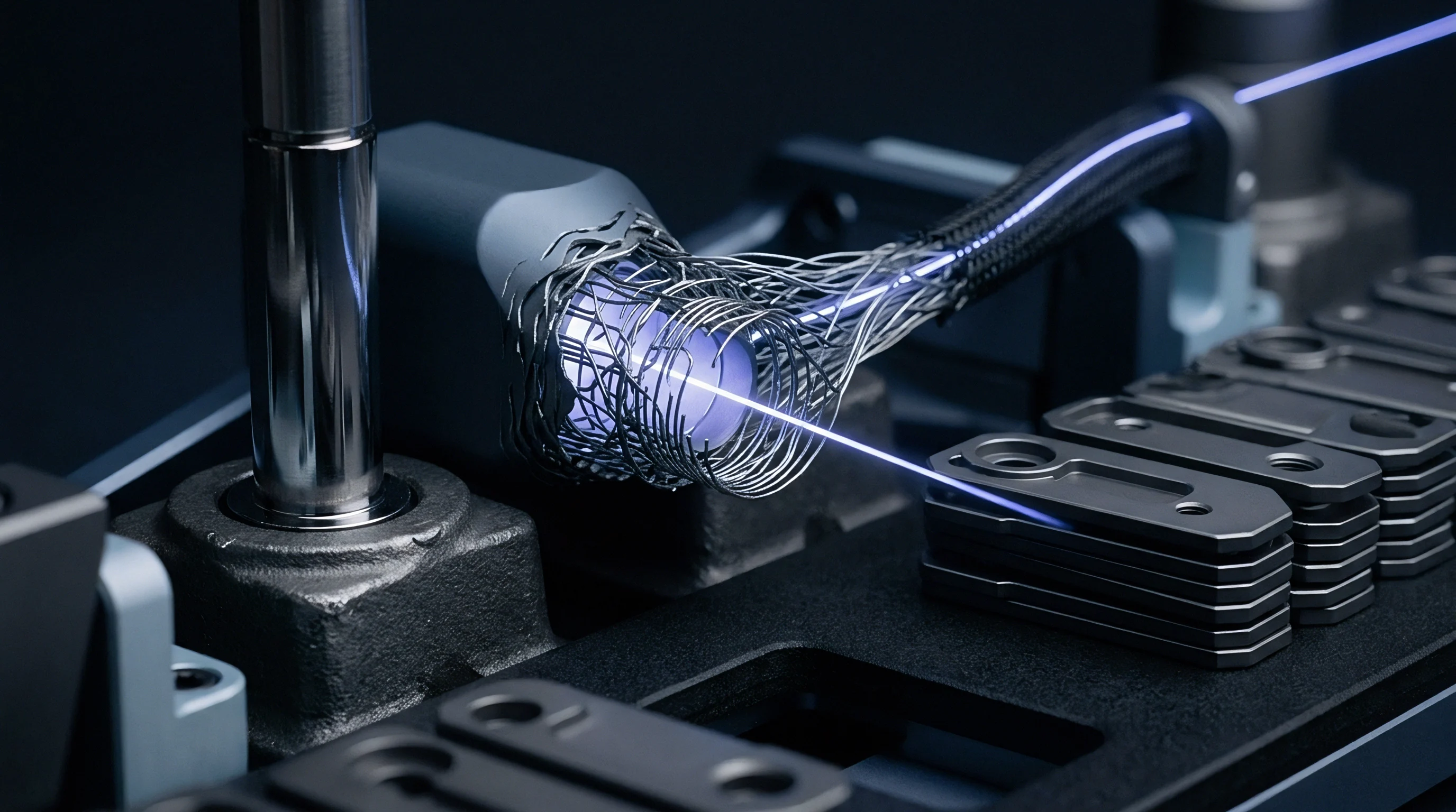
Quadrupole
Winding geometry provides the primary physical defense against transient thermal phase errors. Because the spatial weighting function (2 z – L) is anti-symmetric around the midpoint, winding patterns aim to place fiber segments located equidistant from the center into identical thermal environments. Perfect thermal symmetry forces the spatial integral to zero regardless of the external temperature rate.
A simple dipolar winding pattern alternates single layers from opposite ends of the spool. This configuration provides basic compensation against axial gradients, but remains susceptible to radial thermal fluxes. Quadrupole winding pairs layers symmetrically from the center of the fiber outward.
The wind starts at the fiber center, depositing two layers from one half of the fiber, followed by two layers from the opposite half, alternating in a continuous four-layer sequence until reaching the outer diameter.
Octupole and hexadecapole geometries extend this pairing scheme to eight-layer and sixteen-layer symmetric groups. These higher-order configurations suppress radial and axial gradients by multiple orders of magnitude compared to standard winding. However, increasing the layer grouping order escalates manufacturing difficulty, introduces inter-layer crossover stress, and elevates production scrap rates.
| Winding Architecture | Layer Grouping | Asymmetry Attenuation Ratio | Crossover Sites per Layer | Manufacturing Scrap Rate | Residual Drift (deg/h per K/min) |
|---|---|---|---|---|---|
| Simple Orthocyclic | Single continuous | 1.0 | 1 | < 2% | 120.0 to 450.0 |
| Standard Dipolar | 2-layer alternating | 45.0 | 2 | 3% to 5% | 2.5 to 8.0 |
| Standard Quadrupole | 4-layer symmetric | 650.0 | 4 | 8% to 12% | 0.02 to 0.08 |
| Precision Octupole | 8-layer symmetric | 2800.0 | 8 | 18% to 25% | 0.005 to 0.015 |
| Hexadecapole Array | 16-layer symmetric | 5200.0 | 16 | 35% to 45% | 0.002 to 0.006 |
Geometric imperfections undermine ideal theoretical cancellation. Automated winding machines distribute optical fiber with finite mechanical precision, leaving small discrepancies between paired turns.
System designers categorize winding defects into several reproducible physical failure modes:
- Layer crossover bunching creates localized geometric bulges that displace adjacent turns radially by up to sixty micrometers, degrading symmetry.
- Winding tension variations alter the baseline glass refractive index along the fiber length, preventing complete cancellation of paired segments.
- Potting adhesive voids introduce localized air pockets that drop thermal conductivity by an order of magnitude across specific turn segments.
- Flange proximity skew subjects the outer turns of a layer to increased conductive heat transfer relative to turns resting against the hub.
Axial gradients generate severe bias. When heat enters through a mounting flange, the axial thermal wave reaches the bottom edge of every winding layer before the top edge. Even within a quadrupole pack, turns paired across radial dimensions do not share identical axial coordinates.
This geometric separation leaves a residual asymmetric length Delta L_asym that responds directly to axial temperature rates.
Selecting an inadequate winding architecture forces downstream signal processing stages to absorb massive dynamic errors, resulting in permanent platform drift during rapid vehicle ascents or weapons discharge events.

Filter
Real-time algorithmic compensation augments geometric winding symmetry to eliminate residual thermal bias. Because physical winding cannot achieve absolute mathematical symmetry, secondary calibration systems monitor temperature behavior across the coil assembly. Designers mount discrete temperature sensors on the metallic spool casing, the internal hub, and the external protective shielding to track thermal gradients during platform operation.
Finite impulse response regression models and dynamic state estimators process multi-point temperature data to reconstruct the internal gradient profile. A discrete sensor measures local surface temperature T_k(t), but cannot read the temperature of internal turns directly. By modeling the thermal transfer function between the external surface and the buried fiber layers, digital signal processors synthesize an estimate of the instantaneous Shupe phase rate.
The processing core subtracts this calculated rate error from the raw demodulated Sagnac phase reading at sample rates between one hundred and one thousand hertz.
Thermistor placement dictates model accuracy. Placing sensors solely on the outer housing neglects delayed internal heat accumulation. Optimal configurations distribute thin-film platinum resistance detectors or calibrated semiconductor elements across both axial flanges and the inner spool hub.
Calibration coefficients shift across thermal cycles.
| Compensation Method | Sensor Count | Processing Latency | Dynamic Error Attenuation | Calibration Matrix Size |
|---|---|---|---|---|
| Static Temperature Polynomial | 1 Sensor | < 0.1 ms | 3x to 5x | 4 to 8 Coefficients |
| Multi-Point Gradient Mapping | 4 Sensors | 0.5 to 1.0 ms | 15x to 25x | 32 to 64 Coefficients |
| Discrete Finite Impulse Response Filter | 4 Sensors | 1.5 to 3.0 ms | 40x to 80x | 128 Tap Weights |
| State-Space Thermal Observer | 6 Sensors | 2.0 to 5.0 ms | 100x to 250x | 16 Dynamic States |
System integrators verify compensation performance using dynamic rate tables enclosed in environmental test chambers. Protocols defined in IEEE Std 952 establish formal acceptance testing for single-axis and multi-axis interferometric fiber gyroscopes. Test cycles execute controlled thermal ramps across operating bands spanning minus fifty-five to plus eighty-five degrees Celsius while measuring uncommanded bias wander.
Evaluation of thermal stability typically relies on a standard verification checklist:
- Sensor response calibration verifies that all monitoring thermistors match thermal time constants within two percent of adjacent structural materials.
- Dynamic ramp qualification records gyro drift rates under continuous five kelvin per minute temperature transitions across full operating ranges.
- Spatial gradient characterization evaluates sensor bias stability when external heating blankets apply asymmetric heat flux to individual housing faces.
- Thermal shock recovery tracks the time required for bias readings to return within specified tactical limits following fifty-kelvin fluid submersion steps.
Thermal chamber verification costs often match coil winding expenses. If dynamic modeling coefficients are derived over narrow temperature bands, compensation routines diverge when exposed to non-linear transitions outside the calibration envelope. Long-term aging alters the viscoelastic properties of potting adhesives, shifting thermal diffusion rates and misaligning digital filter taps over multi-year deployments.
Contracts governing navigation payloads specify that transient thermal rate bias must conform to IEEE Std 952 Annex C, defining allowable residual errors below 0.05 degrees per hour under maximum specified operational temperature gradients.