Ground Alignment Metrics for Inertial Sensor Bias Drift Estimation
Static ground alignment accuracy depends on isolating Earth rotation rate from sensor bias instability through multi-position indexing and Allan variance metrics.


Slab
Static positioning of an inertial measurement unit on a stationary mounting fixture forms the foundation of initial bias estimation. Before a navigation platform moves, the physical sensors inside register two constant environmental inputs: Earth’s gravitational acceleration vector and the turn rate vector from planetary rotation. Accelerometers measure local gravity directly, while gyroscope bias dominates horizontal heading drift.
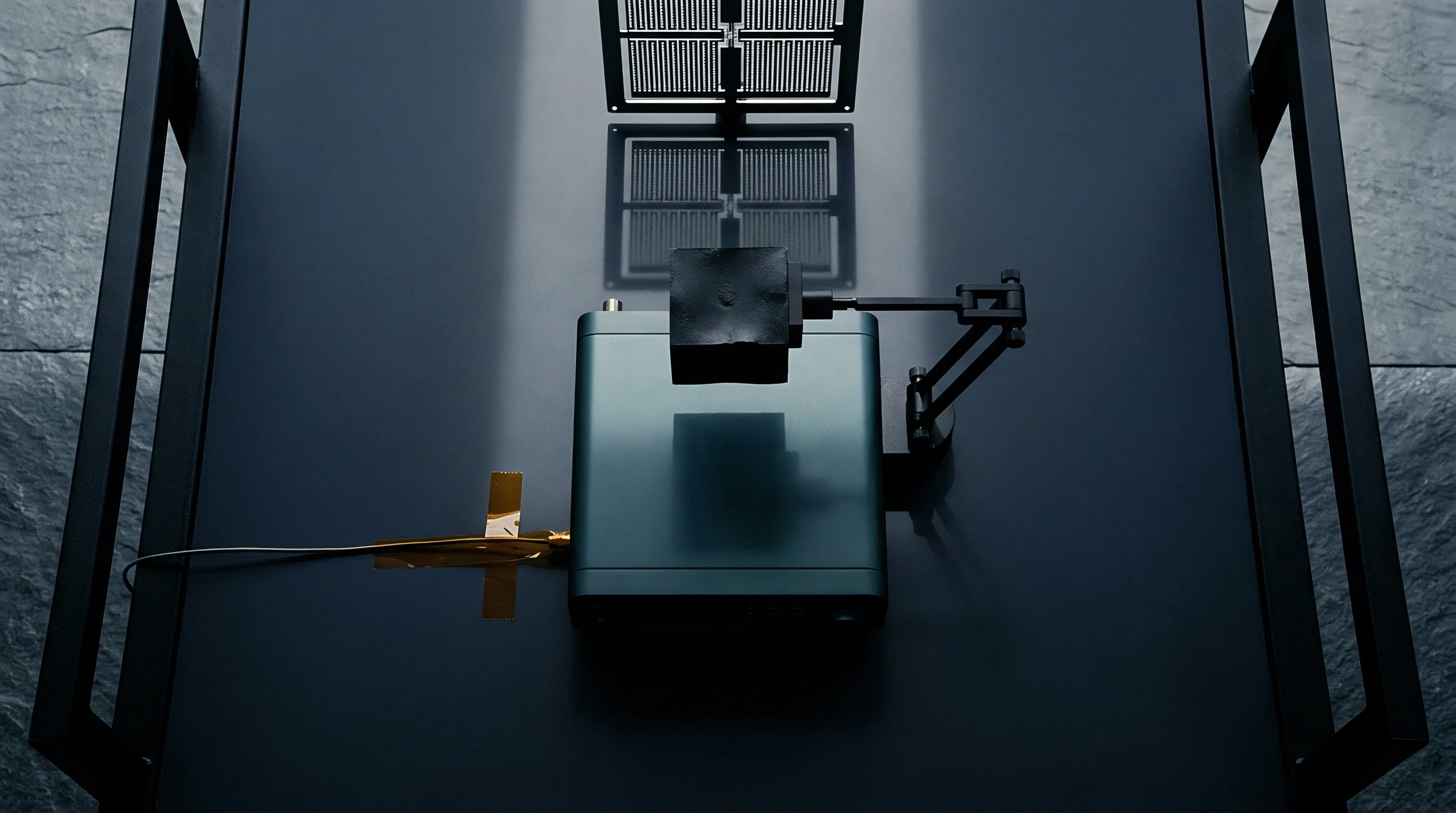
Sitting motionless on a concrete pier isolated from facility vibration, these constant physical inputs establish baseline observability bounds for separating sensor offsets.
Ground alignment algorithms use stationary physics to separate deterministic sensor bias from random stochastic drift. Gravity provides a three-dimensional reference vector with a nominal magnitude of 9.80665 meters per second squared, varying locally with latitude and elevation. The Earth rotates at fifteen degrees per hour.
By measuring how individual accelerometer channels respond to gravity while gyroscopes measure planetary rotation, ground alignment logic calculates initial roll, pitch, and true heading angles. Any residual discrepancy between measured signals and known physical constants is attributed to sensor bias, scale factor error, or axis non-orthogonality.

Earth Rate Isolation and Static Vector Sensing
Gravity serves as the primary reference vector for initial accelerometer leveling. When an inertial measurement unit sits horizontal, its z-axis accelerometer senses full gravitational acceleration while the x and y axes ideally read zero. In practice, real sensors register small offset voltages or digital words on horizontal channels.
These readings define initial tilt angles relative to the local level plane, meaning pitch and roll alignment errors directly reflect any accelerometer bias left unassigned during static initialization.
Sensing Earth’s rotation rate poses a much tougher transducer challenge than sensing gravity. Planetary spin projects a horizontal rotation vector component equal to fifteen point041 degrees per hour multiplied by the cosine of local latitude. At forty-five degrees latitude, this projection comes to roughly ten point63 degrees per hour.
Tactical-grade micro-electromechanical systems gyroscopes, with bias instability floors between one degree and five degrees per hour, resolve this vector only after long static averaging windows. By contrast, fiber optic and ring laser gyroscopes with bias drift below point zero one degrees per hour isolate true north within seconds on a static bench.
Ground tilt distorts horizontal gravity projections. An uncompensated tilt of one arcminute leaks roughly two point85 milligals of gravitational acceleration into horizontal accelerometer channels. If an alignment algorithm misinterprets this tilt as sensor bias, horizontal position drift accumulates quadratically over time.
Disentangling physical mounting tilt from sensor zero-g offset calls for independent optical tilt sensors, liquid leveling references, or multi-position tumbling routines on the pier.

Zero Velocity Observations and Bias Observability
A stationary platform freezes spatial motion, leaving sensor offset drift as the primary driver of integrated velocity accumulation. Zero-velocity update procedures hinge on the known condition that physical velocity is zero. When integrated acceleration yields a non-zero velocity output while resting on the ground, the Kalman filter calculates state corrections to update accelerometer bias estimates.
Mathematically, horizontal gyro bias observability connects directly to horizontal accelerometer bias accuracy through gravity vector cross-coupling.
Azimuth alignment accuracy depends strictly on gyroscope east-axis bias uncertainty. The mathematical bound governing ground gyrocompassing heading error follows a simple trigonometric relationship: residual azimuth error equals east gyroscope bias divided by the product of Earth rotation rate and the cosine of local latitude. At mid-latitudes, an east-axis gyro bias of point zero five degrees per hour produces an azimuth alignment uncertainty of about sixteen arcminutes.
Integrators who miscalculate this bound face severe position drift once mobile operations commence.
Conditioned room air at twenty-one degrees Celsius with velocity under point one meters per second prevents localized sensor thermal gradients during static alignment.
The duration of static initialization limits how cleanly biases can be separated. Short alignment windows under thirty seconds miss low-frequency sensor noise, causing the estimation filter to blend bias instability with high-frequency angle random walk. Extending static dwell time past ten minutes lets long-term flicker noise and thermal drift slip into measurement channels, degrading covariance matrix stability.
The optimal static alignment period balances short-term white noise averaging against long-term sensor drift inflection points.
Evaluations of static baseline performance across several sensor grades mounted on a vibration-isolated pier showed clear thermal limits. During bench trials, thermal hysteresis shifted accelerometer bias by 120 micro-g over a twenty-degree span, corrupting initial pitch leveling by point four arcminutes before thermal equilibrium settled across the aluminum mounting block. Evaluating tactical measurement modules requires checking raw time-series outputs before internal firmware filtering occurs.
Skipping that raw check risks masking high-frequency mechanical resonances under artificial moving averages.
Platform stability during ground alignment dictates how precisely sensor drift parameters can be estimated. Concrete slabs anchored directly to bedrock damp structural flexure, whereas upper floors in industrial facilities transmit low-frequency sway between point two Hertz and three Hertz. This structural motion modulates gravity and Earth rate vectors, introducing artificial noise that corrupts bias convergence.
Engineers quantifying sensor performance specify baseline pier displacement limits to prevent ambient building motion from corrupting vendor acceptance testing.
The desk absorbed a twelve-thousand-dollar re-calibration cost when an uncalibrated optical bench flexed under thermal cycling, injecting three arcseconds of tilt drift that automated test scripts incorrectly flagged as accelerometer zero-g instability.
Kinematics
Estimating bias drift relies mathematically on rigid-body rotation transformations and linear state-space models. Modern inertial navigation filters express system errors through linearized differential equations, mapping sensor noise, scale factor deviations, and bias instabilities into position, velocity, and attitude uncertainties. Estimating bias under static ground conditions demands rigorous covariance matrix formulations to prevent state divergence and cross-axis error coupling.
State vectors in ground alignment filters track core sets of navigation errors. A baseline nine-state filter covers three position errors, three velocity errors, and three attitude misalignments. Expanding to fifteen states incorporates three accelerometer biases and three gyroscope biases.
When high-accuracy performance requires extra state resolution, engineers add scale factor stability and non-orthogonality parameters, creating a twenty-one-state system model that requires full observability verification under static constraints.

Covariance Matrix Dynamics in Tilt and Azimuth Estimation
Linearized error propagation models map sensor noise parameters directly into attitude uncertainty states. During static ground alignment, the system observation model compares integrated inertial outputs against zero velocity measurements. Subtracting predicted zero velocity from integrated accelerometer counts yields an innovation sequence that drives state updates across the covariance matrix.
Horizontal velocity residual signals update pitch and roll estimates, while vertical channel residuals adjust vertical bias terms.
Uncertainty in horizontal accelerometer bias directly degrades level alignment. Cross-covariance terms between accelerometer bias states and attitude error states dictate how fast the filter transfers observed velocity errors into sensor corrections. If initial covariance values assigned to accelerometer biases are set unrealistically low, the Kalman filter ignores velocity residuals and attributes position drift entirely to attitude error.
Proper tuning matches state covariance values to verified Allan variance drift metrics.
Azimuth alignment covariance converges far slower than pitch and roll covariance states. Pitch and roll states update directly from large gravity vector projections on horizontal axes, settling within seconds. Azimuth alignment relies instead on measuring small Earth rotation rate projections on horizontal gyroscopes.
Because Earth rate is small relative to tactical MEMS noise floors, reducing azimuth covariance demands extended stationary observation periods or multi-position mechanical rotations.
Allan Variance Breakdown for Static Bias Extraction
Time-domain stochastic analysis separates high-frequency noise elements from long-term sensor drift. Standardized under IEEE 952 for gyroscopes and IEEE 1431 for accelerometers, Allan variance analysis calculates sample variances of averaged time-series data across varying cluster times. Plotting Allan deviation against cluster duration on logarithmic scales yields distinct slope regions that identify specific physical noise mechanisms operating within the transducer die and readout electronics.
Quantization noise dominates short cluster times, appearing as a minus-one slope on the Allan deviation plot. As cluster duration increases, angle random walk for gyroscopes and velocity random walk for accelerometers emerge, characterized by a minus one-half slope. Angle random walk reflects high-frequency white noise originating from mechanical thermal agitation inside MEMS structures or photon shot noise inside optical gyroscopes.
Ground alignment algorithms integrate through this noise region to extract underlying deterministic biases.
Bias instability defines the flat, zero-slope region of the Allan deviation curve, representing the fundamental limit of sensor drift predictability. This flicker noise floor sets the lowest bias uncertainty achievable through static ground averaging. Beyond the bias instability minimum, rate random walk (a plus one-half slope) and linear drift ramps (a plus one slope) signal long-term environmental degradation, thermal shifts, and strain relaxation.
Ground alignment metrics isolate the bias instability cluster time to set optimal stationary observation windows.
| Sensor Grade Class | Gyro Bias Instability (deg/hr) | Angle Random Walk (deg/sqrt-hr) | Accel Bias Instability (micro-g) | Velocity Random Walk (m/s/sqrt-hr) | Static Gyrocompassing Time (min) |
|---|---|---|---|---|---|
| Consumer MEMS | 10.0 to 50.0 | 0.50 to 2.00 | 500 to 2000 | 0.200 to 0.800 | Not Applicable |
| Industrial MEMS | 1.0 to 5.0 | 0.05 to 0.20 | 50 to 200 | 0.030 to 0.100 | 60 to 120 |
| Tactical MEMS | 0.05 to 0.50 | 0.008 to 0.030 | 10 to 50 | 0.005 to 0.020 | 15 to 30 |
| Navigation FOG | 0.001 to 0.010 | 0.0005 to 0.0020 | 1 to 5 | 0.0008 to 0.0030 | 2 to 5 |
| Strategic RLG | 0.0001 to 0.0008 | 0.0001 to 0.0003 | 0.1 to 1.0 | 0.0001 to 0.0005 | 0.5 to 1.5 |
Extracting bias parameters mathematically during ground alignment runs into physical limits set by sensor noise metrics. Key physical error mechanisms that corrupt bias observability during stationary passes include:
- Angular Random Walk Phase Shift High-frequency broadband noise introduces pseudo-random integration drift that mimics short-term zero offset changes over short alignment windows.
- Temperature-Dependent Offset Drift Thermal gradients across sensor silicon substrates shift active piezoresistive or capacitive bridge output balances during static initialization.
- Scale Factor Asymmetry Distortion Discrepancies between positive and negative output gains produce non-linear rectification signals when small bench vibrations pass through sensor channels.
- Cross-Axis Coupling Rectification Structural non-orthogonality between transducer mechanical axes couples gravity vectors directly into horizontal sense channels during static leveling.
Standard IEEE 952 specifies that angle random walk and bias instability be extracted from uncompensated Allan variance plots without low-pass digital filtering.
Uncalibrated gyro scale factor error degrades static bias estimation when the sensor platform undergoes indexing rotations. If a two-axis tilt table rotates an IMU ninety degrees to isolate horizontal biases, scale factor errors scale the Earth rotation signal, creating an artificial bias term. Separating scale factor errors from zero-rate offsets requires multi-position inversion techniques where sensors undergo full 180-degree physical reversals relative to the Earth rate vector.
State estimation filters can become numerically unstable when sensor noise covariance matrices contain ill-conditioned values. When high-precision fiber optic gyroscopes partner with low-cost capacitive accelerometers, the variance ratio between state channels exceeds six orders of magnitude. Square-root Kalman filtering algorithms and U-D factorization prevent precision loss and matrix singularity during long ground alignment runs, preserving numerical stability across thirty-two-bit floating-point DSP platforms.
Procurement specifications rely on verified Allan deviation parameters rather than simple peak-to-peak noise ratings. Peak-to-peak metrics hide spectral noise distribution details, masking high-frequency quantization noise that degrades Kalman filter innovation sequences. Examining the log-log slope of sample variance reveals whether an inertial module will settle cleanly during ground alignment or wander indefinitely due to uncompensated random walk.
How do low-frequency floor vibrations couple into vertical accelerometer channels to alter static zero-g bias estimation stability?

Vibration
Mechanical disturbance energy passing through test fixtures alters sensor output signals during baseline measurements. Environmental floor movement, HVAC mechanical noise, and acoustic excitation transmit directly through mounting brackets into sensitive MEMS silicon structures and optical fiber coils. Ground alignment algorithms that assume absolute physical stillness mistake vibration-induced rectification for sensor bias drift, skewing initial state convergence.
Dynamic cross-axis sensitivity ~ known as g-sensitivity in gyroscopes and vibro-pendular error in accelerometers ~ converts high-frequency mechanical oscillation into artificial DC offset shifts. When a MEMS capacitive accelerometer experiences high-frequency vibration along its flexure axis, non-linear electrostatic forces generate a rectified DC acceleration signal. This artificial offset persists for as long as mechanical excitation continues, masking true zero-g bias during static ground calibration.

Does Base Seismic Activity Limit MEMS Bias Calibration?
Microseism motion originating from ocean waves and industrial equipment creates low-amplitude bench displacement. Operating between point one Hertz and point five Hertz, ambient seismic background vibration induces tilt oscillations ranging from point one to two arcseconds peak-to-peak. While imperceptible to human operators, these low-frequency tilt variations produce horizontal acceleration signals up to ten micro-g.
Tactical MEMS sensors designed to estimate zero-g bias within five micro-g capture this seismic motion as real signal input, blurring zero-offset identification.
Acoustic pressure waves generated by cooling fans and bench equipment excite local structural modes in thin-walled sensor enclosures. Sound pressure levels exceeding seventy decibels at frequencies near MEMS structural resonance modes disrupt internal comb-drive sense elements. This acoustic coupling shifts gyroscope output baselines by several degrees per hour.
Installing sound-dampening acoustic enclosures around bench fixtures eliminates atmospheric pressure wave coupling during precision ground alignment runs.
Seismic base movement degrades horizontal gyroscope alignment precision whenever floor velocity noise exceeds sensor bias drift rates.
Isolating ground test stations from ambient mechanical noise requires dedicated structural engineering solutions. Heavy optical tables resting on pneumatic air springs damp vibrations above five Hertz, reducing floor displacement transmission by up to thirty decibels. However, pneumatic suspension systems introduce low-frequency table rocking modes around one Hertz.
Alignment filters must notch-filter these isolation table resonance frequencies to prevent artificial low-frequency oscillations from corrupting bias drift metrics.
The checklist below outlines operational engineering measures required to isolate ground alignment test benches from external mechanical disturbances.
- Bedrock Pier Coupling Verification Anchoring concrete mounting blocks directly to sub-floor bedrock isolates test fixtures from building mechanical plant vibrations.
- Pneumatic Suspension Tuning Adjusting air table damping valves eliminates sub-Hertz table sway modes that introduce false horizontal acceleration signals.
- Acoustic Enclosure Isolation Shielding sensor hardware with heavy density mass-loaded vinyl dampens airborne sound pressure waves near MEMS resonant frequencies.
- Cable Strain Relief Installation Securing signal and power wiring to isolated fixtures prevents mechanical cable tension from transmitting vibration to sensor housings.

Thermal Gradients and Mounting Strain Signals
Temperature shifts across sensor housings induce internal mechanical stresses that shift zero-input offsets. Differentials in thermal expansion coefficients between silicon sensor dies, ceramic substrates, printed circuit boards, and aluminum housings strain internal sense elements. This strain alters piezoresistive bridge resistances and changes capacitive plate gaps, shifting output voltages independently of physical rotation or acceleration.
Spatial thermal gradients across an inertial housing prove far more destructive to bias stability than uniform ambient temperature changes. A spatial temperature difference of point five degrees Celsius across a tactical fiber optic gyroscope coil creates non-symmetric phase shifts in counter-propagating light beams via the Shupe effect. This thermal gradient generates an artificial bias shift exceeding one degree per hour.
Symmetrical packaging design and thermal insulation shrouds minimize internal spatial gradients during ground alignment.
Stationary benches still vibrate continuously, demanding strict limits on ambient bench vibration before attempting any gyrocompassing verification procedure. Unfiltered floor vibration at twelve Hertz passed through an un-damped aluminum fixture during early bench testing, rectifying into a seventy-micro-g DC bias shift across horizontal accelerometer channels. Incorporating elastomer isolation dampers reduced high-frequency vibration transmission, restoring true zero-g bias readings within vendor specification limits.
Bench cooling fan air currents striking an unsealed sensor housing during baseline calibration cycles can induce false static drift exceedances during factory testing.
Validation
Empirical bench testing confirms theoretical sensor error models before units are integrated into guidance assemblies. Automated test routines isolate deterministic bias offsets, scale factor coefficients, and non-orthogonality matrices from stochastic noise floors. Establishing standardized verification protocols guarantees that sensor units satisfy baseline ground alignment tolerances under physical bench testing before deployment into high-stress operational environments.
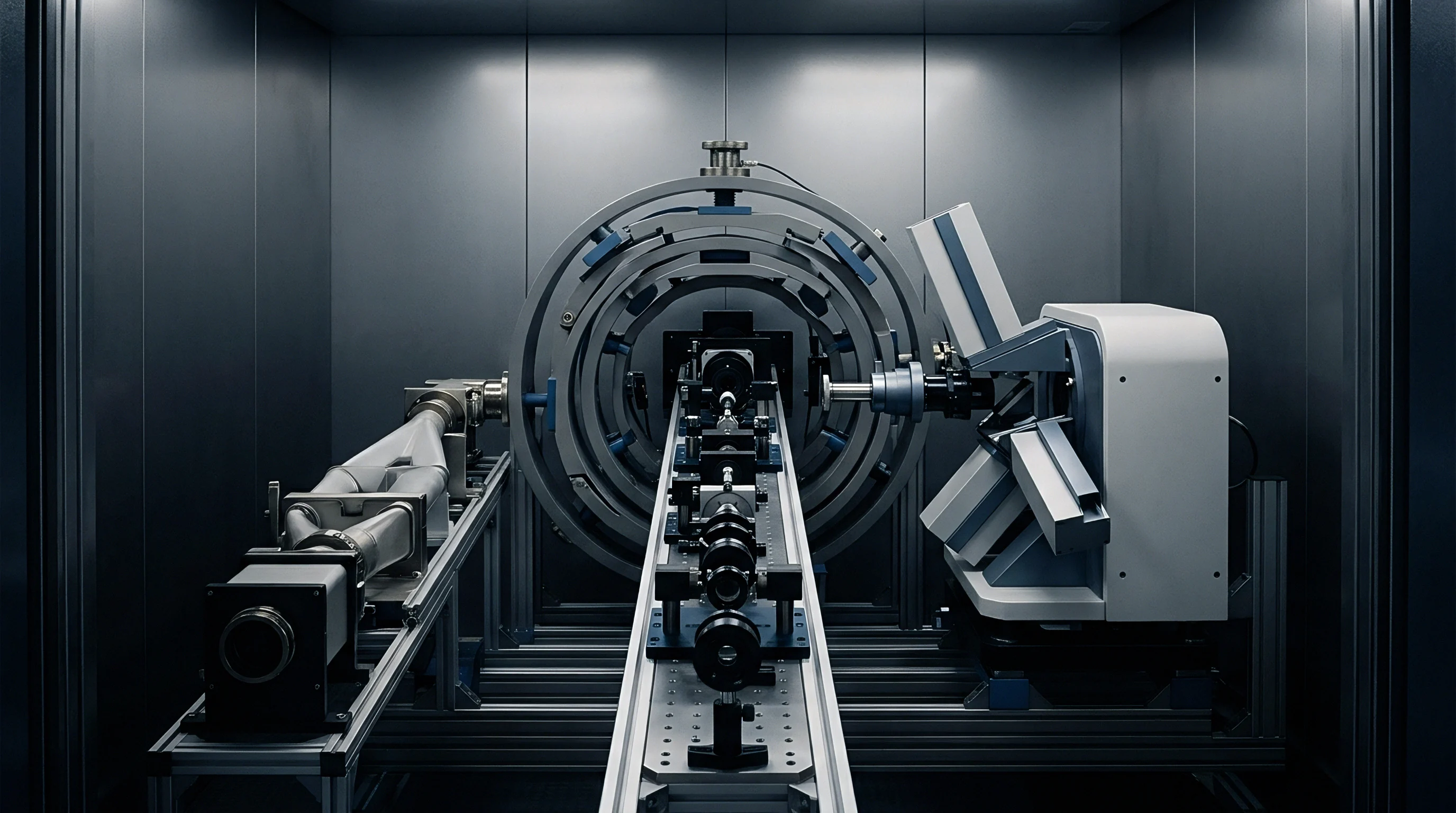
Multi-axis rate tables with positioning accuracy under two arcseconds provide the gold standard physical reference for inertial calibration. Precision optical encoders track table axis position while temperature-controlled chambers regulate ambient thermal conditions. Mounting inertial packages inside these automated test systems allows engineers to execute programmed rotation and static dwell sequences that separate gravity vectors and Earth rate signals from internal sensor errors.
Multi Position Indexing Protocols for Inertial Profiling
Precise physical rotation of sensor hardware through known orthogonal angles isolates offset bias from scale factor error. The classic six-position tumbling test rotates an inertial measurement unit through positive and negative orientations along three orthogonal axes. In each position, one accelerometer axis aligns directly with gravity while the remaining two axes rest perpendicular to the gravity vector.
Summing output readings from opposing 180-degree orientations cancels scale factor errors, exposing true zero-g bias offsets.
Advanced calibration routines utilize twelve-position or twenty-four-position indexing sequences to isolate cross-axis non-orthogonality and scale factor non-linearity. By rotating the sensor package through forty-five-degree tilt increments, test algorithms map non-linear transducer responses across full operational ranges. The mathematical system of equations generated by multi-position testing forms an over-determined linear system solved via least-squares regression to extract individual bias vector components.
The step-by-step procedure below details the execution sequence for a six-position static tumbling test used to extract accelerometer zero-g bias offsets.
- Mount the inertial sensor package securely onto the optical index plate of a calibrated multi-axis rate table.
- Allow the sensor package to achieve thermal equilibrium inside the environmental chamber at twenty-five degrees Celsius for sixty minutes.
- Record raw output counts across all accelerometer channels during a ten-minute static dwell in the baseline horizontal position.
- Rotate the primary table axis 180 degrees to invert the sensor package and record static output data for an additional ten-minute dwell.
- Repeat the 180-degree rotation and ten-minute static dwell sequence across the remaining two orthogonal axes.
Multi-axis indexing turn-tables eliminate earth rate vector cross-talk when rotation axes maintain perpendicularity within ten arcseconds.
Thermal Chamber Dwell and Residual Extraction Metrics
Controlled environmental testing evaluates how bias stability degrades when ambient temperature varies across operational ranges. Environmental chambers execute controlled thermal ramps from minus forty degrees Celsius to plus eighty-five degrees Celsius while sensors hold static orientations on rate table mounts. Soaking the sensor package at fixed temperature steps isolates steady-state thermal bias coefficients from dynamic thermal gradient transient responses.
Polynomial compensation models fit thermal bias data recorded during chamber testing. Third-order polynomial equations map sensor housing temperature inputs to predicted bias correction terms calculated real-time inside system firmware. The residual bias metric evaluates calibration quality by measuring the remaining uncompensated bias offset after polynomial thermal corrections are applied across the entire temperature operating window.
| Calibration Method | Static Dwell Time (min) | Residual Accel Bias (micro-g) | Residual Gyro Bias (deg/hr) | Azimuth Error Bound (arcmin) | Thermal Compensation Degree |
|---|---|---|---|---|---|
| Single-Position Static Dwell | 5.0 | 250 | 2.50 | 45.0 | None (Raw Signal) |
| Six-Position Static Tumble | 30.0 | 45 | 0.35 | 8.0 | 1st Order Linear |
| Twelve-Position Indexing | 60.0 | 15 | 0.08 | 2.2 | 2nd Order Polynomial |
| 24-Position Multi-Thermal | 240.0 | 3 | 0.01 | 0.4 | 3rd Order Spline |
Evaluating residual bias performance demands long-term continuous testing to ensure model validity. Quality assurance rejects sensor lots when static drift exceeds allowable thresholds during initial room-temperature screening. Inspecting residual bias distributions across production batches highlights manufacturing defects, such as die-attach micro-cracking or wire-bond strain relaxation, that manifest as step-change bias instabilities during thermal cycling.
According to clause four point two of IEEE standard 1431, accelerometer bias repeatability across un-powered thermal cycles dictates the minimum recalibration interval for tactical navigation units.
Ledger
Procurement records and bill-of-materials specifications dictate the economic viability of selecting specific inertial sensor grade tiers. Balancing unit acquisition pricing against downstream calibration costs forms the core financial decision when specifying inertial hardware for high-volume production. Selecting high-performance optical sensors increases upfront component expense while reducing field calibration requirements, whereas low-cost MEMS components demand extensive factory calibration and complex ground alignment software to satisfy system requirements.
Landed sensor costs reflect far more than the bare component purchase order price. Wafer-level MEMS packaging reduces initial component purchase costs to tens of dollars, but validating these components requires automated rate tables, thermal chambers, and extended test durations that add significant production overhead. High-end fiber optic gyroscopes incur high initial component procurement costs but land with pre-calibrated factory bias matrices, minimizing downstream assembly line test time.
Datasheet Performance Bounds versus Bench Verification
Manufacturer component specifications often present optimal baseline figures recorded under idealized bench conditions. Datasheet bias stability claims typically reflect ninety-five percent confidence limits taken at room temperature in vibration-isolated laboratories over short cluster windows. System integrators who accept these figures without independent verification discover that operational ground alignment performance degrades significantly under real-world ambient conditions.
Specifying bias parameters for procurement contracts requires clear definitions of test conditions and statistical boundaries. A datasheet claiming zero-g bias stability of ten micro-g must specify whether that figure represents short-term Allan variance minimums, long-term turn-on to turn-on repeatability, or residual errors across full thermal ranges. Vague vendor claims mask underlying instabilities that require costly software workarounds during integration phases.
| Transducer Technology | Unit Cost (USD) | Lead Time (Weeks) | Verified Gyro Bias (deg/hr) | Turn-on Repeatability (deg/hr) | Qualification Standard |
|---|---|---|---|---|---|
| Consumer Capacitive MEMS | 2 to 15 | 6 to 10 | 15.0 to 50.0 | 25.0 | AEC-Q100 Grade 3 |
| Industrial MEMS Module | 150 to 500 | 12 to 16 | 1.5 to 5.0 | 3.0 | AEC-Q100 Grade 1 |
| Tactical Quartz / MEMS | 1,500 to 4,500 | 16 to 24 | 0.10 to 0.50 | 0.25 | MIL-STD-810H |
| Closed-Loop FOG | 8,000 to 18,000 | 24 to 36 | 0.005 to 0.020 | 0.010 | DO-160G Class S2 |
| Monolithic RLG Assembly | 25,000 to 60,000 | 32 to 52 | 0.0005 to 0.0020 | 0.0010 | MIL-PRF-27105D |
Commercial Sourcing and Qualification Requirements
Component selection decisions balance sensor unit pricing against downstream calibration infrastructure costs. Securing reliable second-source suppliers for tactical-grade inertial measurement units presents substantial commercial challenges. Silicon MEMS foundries utilize proprietary etching processes and custom application-specific integrated circuits that make pin-for-pin cross-qualification impossible without redesigning host processing boards and ground alignment firmware.
Sole-source supplier exposure poses severe financial risks during global supply chain disruptions. Alternate part qualification requires four to six months of environmental testing, rate-table profiling, and field verification flights to prove equivalent bias stability. System architects hedge supply risks by designing modular sensor interfaces that accept standardized digital communication protocols and generic error state models across multiple vendor components.
Sourcing decisions lock in long-term supply risk. Uncalibrated drift ruins position accuracy, and bench testing often exposes unquoted thermal hysteresis. When writing request-for-quotation documents, engineering teams demand raw time-series test data, full thermal calibration matrices, and Allan variance plots recorded across minimum sample sizes of thirty units per manufacturing lot.
High production calibration costs signal an unstable sensor packaging process.