Basic Noise Spectral Density Conversions for Sensor Front Ends
Root sum square integration of spot noise spectral density across effective noise bandwidth determines actual sensor resolution and achievable effective bits.
Band
Transducer datasheets express internal physical disturbances as spectral densities normalized to a single Hertz interval. Expressing random fluctuations as voltage spectral density in nanovolts per root Hertz or current spectral density in picoamperes per root Hertz decouples the intrinsic noise floor of the sensing element from the downstream filter bandwidth. This continuous spectral density represents the square root of the power spectral density across a theoretical one Hertz wide band.
Evaluating physical sensor signals requires converting these spot density figures into root-mean-square and peak-to-peak voltage amplitudes that match the input range of an analog-to-digital converter.
Thermal fluctuations govern conductors. Johnson-Nyquist thermal noise arises from the microscopic thermal agitation of charge carriers inside resistive materials. The thermal voltage spectral density of a passive resistive element follows the physical relation where voltage noise density equals the square root of four times Boltzmann’s constant, absolute temperature in Kelvin, and resistance in Ohms.
At room temperature of 298 Kelvin, a 10 kiloohm sensor source impedance generates a thermal voltage noise density of 12.8 nanovolts per root Hertz. Lowering source resistance reduces thermal noise, but physical transduction mechanisms impose lower limits on active sensor element impedance.
Spot Noise Spectral Density Foundations
Voltage variations inside physical elements stem directly from thermal fluctuations and charge quantum discrete arrivals. Current noise density arises primarily from shot noise, generated when electrical current crosses potential barriers such as semiconductor junctions. Shot noise current spectral density equals the square root of two times elementary electron charge multiplied by direct bias current in Amperes.
A sensor bias current of 1 milliampere produces a shot noise current spectral density of 17.9 picoamperes per root Hertz. Shot noise tracks current.
Sensor element impedance dictates whether current noise spectral density or voltage noise spectral density dominates front-end signal degradation.
High-impedance sensor elements such as piezoelectric crystals, glass pH electrodes, and unamplified photodiodes translate current noise spectral density directly into large terminal voltage fluctuations across their output impedance. Conversely, low-impedance transducers like strain gauge bridges and thermocouple junctions are limited almost exclusively by voltage noise spectral density and thermal source resistance. Matching the analog front-end operational amplifier to the sensor demands balancing amplifier input voltage noise density against amplifier input current noise density multiplied by sensor source impedance.
Transducer Specific Density Characteristics
Photodiodes operating in photovoltaic mode exhibit shot disturbance proportional to dark current leakage. Capacitive Micro-Electro-Mechanical Systems acceleration transducers generate equivalent noise spectral density through mechanical Brownian damping of the internal proof mass. Piezoelectric pressure sensors produce charge spectral density that must be conditioned through low-leakage charge amplifiers.
Measuring each modality requires establishing the dominant noise mechanism before dimensioning active conditioning stages.
| Sensor Modality | Dominant Noise Mechanism | Typical Source Impedance | Voltage Spectral Density | Current Spectral Density |
|---|---|---|---|---|
| Photodiode Transimpedance | Dark Current Shot Noise | 10 MΩ to 1 GΩ | 1.2 nV/√Hz | 0.08 pA/√Hz |
| Piezoelectric Charge | Dielectric Loss & Brownian | 100 MΩ (Capacitive) | 4.5 nV/√Hz | 0.01 pA/√Hz |
| Capacitive MEMS | Brownian Air Damping | 1 MΩ (At Resonance) | 12.0 nV/√Hz | 0.005 pA/√Hz |
| Piezoresistive Bridge | Johnson Thermal Resistance | 350 Ω to 5 kΩ | 2.4 nV/√Hz | 1.50 pA/√Hz |
| Data recorded at 25°C ambient temperature with bias conditions specified for standard industrial sensing front ends. | ||||
Quantifying total input-referred noise density involves combining independent noise sources using root-sum-square addition. Independent random noise signals do not sum algebraically; their power spectral densities add linearly. Uncorrelated voltage spectral density components combine by taking the square root of the sum of their squared individual densities.
Neglecting any single secondary noise source that exceeds one-third of the primary noise density introduces unacceptable error into front-end signal-to-noise ratio projections.
- Bandwidth omission ~ Standardizing spectral density without defining the measurement frequency span leads to underestimating high-frequency broadband alias noise.
- Impedance mismatching ~ Converting current noise density directly into voltage without accounting for frequency-dependent sensor impedance creates severe phase-lag calculation errors.
- Corner frequency oversight ~ Applying white noise spectral density down to direct current ignores the 1/f flicker ceiling of active sensor elements.
Sensor front ends operating near physical noise floors maintain precision only when gain stages match transducer impedance boundaries.
Integration
Converting broadband continuous spot values into total output root-mean-square amplitude demands calculating total statistical area under the spectral power curve. Integrated voltage noise equals the input spot noise spectral density multiplied by the square root of the equivalent noise bandwidth. The equivalent noise bandwidth represents the passband frequency of an ideal brick-wall filter that transmits the exact same noise power as the actual analog filter chain.
White noise spectral density remains constant across frequency, making noise power directly proportional to effective bandwidth.
Filter attenuation rolls off smoothly. Realizing a physical single-pole resistance-capacitance low-pass filter with a three-decibel corner frequency of 10 kilohertz does not cut off noise sharply at 10 kilohertz. The gradual attenuation roll-off allows higher frequency noise components to pass through the conditioning chain.
The equivalent noise bandwidth for a first-order low-pass filter equals 1.57 times its three-decibel cutoff frequency. A 10 kilohertz first-order filter has an equivalent noise bandwidth of 15.7 kilohertz.
How Does Filter Order Alter Integrated Noise?
Real analog low-pass stages do not drop off abruptly at their half-power cutoff point. Increasing filter order steepens the attenuation slope above the cutoff frequency, bringing equivalent noise bandwidth closer to the target signal bandwidth. A second-order Butterworth filter possesses a noise bandwidth factor of 1.11 times its three-decibel cutoff frequency.
A third-order filter reduces this factor to 1.05, and a fourth-order filter achieves 1.02. Cascading active filter poles restricts integrated high-frequency noise power without restricting flat passband signal transmission.
Standard specification limits for industrial measurement conditioning require multiplying three-decibel analog bandwidths by filter order coefficients before calculating integrated RMS voltage floors.
Flicker noise dominates DC levels. Low-frequency 1/f noise exhibits a spectral power density that increases inversely with frequency. Calculating integrated root-mean-square voltage within the 1/f region requires integrating the spectral density function from a lower operational frequency limit to an upper cutoff limit.
The resulting equation states that integrated 1/f root-mean-square noise equals the spot noise density measured at 1 Hertz multiplied by the square root of the natural logarithm of the ratio of high cutoff frequency to low cutoff frequency.

Flicker Corner and Crest Factor Scaling
Low-frequency spectral curves rise inversely with frequency until hitting white background floor thresholds. The flicker corner frequency defines the intersection point where 1/f noise density equals white flat-band noise density. When the signal measurement band extends below this corner frequency, total integrated root-mean-square noise must combine both 1/f noise and white broadband noise using root-sum-square addition.
Ignoring 1/f noise contributions in low-frequency sensors such as precision strain balances or temperature monitors causes severe underestimation of total system drift.
Translating root-mean-square noise into peak-to-peak values requires applying statistical crest factors. Gaussian noise voltage distribution implies that peak amplitudes theoretically have no absolute maximum bound. For practical circuit engineering, peak-to-peak noise is defined within statistical probability limits.
Multiplying root-mean-square noise by a crest factor of 6.6 guarantees that the peak-to-peak noise excursion remains within that calculated voltage span for 99.9 percent of operating time. High-reliability instrumentation front ends apply a crest factor of 8.0 to achieve 99.994 percent peak certainty.
- Determine the low-frequency limit and high-frequency corner of the signal chain’s active measurement band.
- Multiply the analog filter cutoff frequency by the filter order factor to obtain the equivalent noise bandwidth.
- Calculate the integrated white noise voltage across the effective noise bandwidth using root power addition.
- Compute the 1/f flicker noise contribution using the natural logarithm ratio of the high and low cutoff limits.
- Combine white noise and flicker noise through root-sum-square addition before multiplying by the crest factor.
Evaluating signal chain resolution relies on converting peak-to-peak noise into effective number of bits. Effective resolution equals the logarithm base two of full-scale input voltage range divided by total peak-to-peak output noise voltage. Alternatively, effective number of bits calculated from signal-to-noise-and-distortion ratio uses the standard converter formula where effective bits equal signal-to-noise ratio minus 1.76 divided by 6.02.
Converting noise spectral density to peak-to-peak voltage establishes the ultimate hardware limitation on achievable data converter resolution.
Failure to integrate non-ideal filter roll-off tails results in undersizing analog-to-digital converter dynamic range specifications and missing critical system resolution targets.
Chain
A concrete signal stage calculation demonstrates how physical source disturbances propagate through amplification and analog-to-digital conversion. Consider a high-impedance piezoelectric sensor front end driving a precision operational amplifier configured as a non-inverting voltage stage feeding a 24-bit delta-sigma converter. The sensor features an internal source resistance of 100 kiloohms at 25 degrees Celsius, producing a thermal noise voltage density of 40.5 nanovolts per root Hertz.
The operational amplifier exhibits an input voltage noise density of 4.0 nanovolts per root Hertz and an input current noise density of 5.0 femtoamperes per root Hertz at 1 kilohertz.
The quoted amplifier input spot noise density of 4.0 nanovolts per root Hertz at 1 kilohertz rests on a manufacturer bench test conducted at 25 degrees Celsius under a 5 Volt supply with a 10 milliampere quiescent current. Operating the same die at 85 degrees Celsius elevates the broadband floor to 4.4 nanovolts per root Hertz due to thermal mobility reduction in the input differential pair. High gain amplifies early noise.
Stage Wise Error Budget Construction
Piezoelectric sensors outputting charge through high-impedance cabling generate primary source thermal voltage fluctuations. Input current noise from the amplifier flows through the 100 kiloohm source resistance, generating an additional voltage noise density component equal to 5.0 femtoamperes per root Hertz multiplied by 100 kiloohms, which yields 0.5 nanovolts per root Hertz. Because this current-induced noise voltage density is far below the sensor thermal noise density of 40.5 nanovolts per root Hertz, source thermal noise dominates the total input spectral density.
Total input-referred spot noise density combines sensor thermal noise, amplifier voltage noise, and current-induced noise. Summing these terms using root-sum-square calculation yields the square root of 40.5 squared plus 4.0 squared plus 0.5 squared, resulting in a total input-referred spot noise density of 40.7 nanovolts per root Hertz at 1 kilohertz. The source resistance accounts for 98.5 percent of total spot noise power at this stage.
| Stage Element | Individual Spot Density | Stage Gain (V/V) | Output-Referred Spot Density | Integrated RMS Noise (100 Hz BW) |
|---|---|---|---|---|
| Sensor Source Resistor (100 kΩ) | 40.5 nV/√Hz | 10.0 | 405.0 nV/√Hz | 5.07 µV rms |
| Op Amp Input Voltage Noise | 4.0 nV/√Hz | 10.0 | 40.0 nV/√Hz | 0.50 µV rms |
| Op Amp Current Noise Density | 0.5 nV/√Hz | 10.0 | 5.0 nV/√Hz | 0.06 µV rms |
| ADC Driver Noise Floor | 12.0 nV/√Hz | 1.0 | 12.0 nV/√Hz | 0.15 µV rms |
| Total Combined System Chain | 42.2 nV/√Hz (Input) | 10.0 | 422.0 nV/√Hz | 5.29 µV rms |
Assuming the front-end amplifier stage is set to a voltage gain of 10, the output-referred noise spectral density becomes 407 nanovolts per root Hertz. Passing this signal through a single-pole low-pass RC filter with a 3-decibel cutoff frequency of 100 Hertz creates an equivalent noise bandwidth of 157 Hertz. Integrating 407 nanovolts per root Hertz over 157 Hertz equivalent noise bandwidth gives a total integrated output voltage noise of 5.10 microvolts root-mean-square.
System signal-to-noise ratio limits remain locked to the primary transduction stage when initial amplifier gain exceeds twenty decibels.
Conversion to Effective Resolution
Peak-to-peak output amplitude sets the smallest discernible physical signal quantum above system floor limits. Multiplying 5.10 microvolts root-mean-square by a crest factor of 6.6 translates the output noise floor to 33.7 microvolts peak-to-peak. Connecting this conditioned output to a 24-bit delta-sigma converter operating with a 2.5 Volt full-scale input span allows evaluating effective noise-free quantization performance.
Noise-free resolution equals the logarithm base two of 2.5 Volts divided by 33.7 microvolts, yielding 16.18 bits. Although the analog-to-digital converter possesses a 24-bit nominal architecture, physical sensor thermal noise and amplifier stage conditioning restrict true noise-free output performance to 16 bits. The remaining 8 lower bits represent random noise fluctuations rather than physical sensor input variations.
Whether chopper-stabilized amplifiers introduce unacceptably high switching charge injection spikes into high-impedance capacitive elements remains a persistent design challenge across dynamic front ends.
Drift
Temperature variations inside operational enclosures shift amplifier bias currents and silicon substrate thermal equilibrium. Thermal noise voltage density increases with the square root of absolute temperature. Heating a sensor front end from 20 degrees Celsius to 85 degrees Celsius increases absolute temperature from 293 Kelvin to 358 Kelvin, causing a 10.5 percent increase in intrinsic Johnson thermal noise density.
Higher ambient temperature elevates baseline noise power independently of active component degradation.
Temperature shifts bias currents. Semiconductor junction leakage current doubles approximately every 10 degrees Celsius rise in silicon operating temperature. JFET and CMOS operational amplifier input bias currents expand rapidly at elevated temperatures, dramatically accelerating current noise spectral density.
A JFET input stage exhibiting 1 picoampere bias current at room temperature can exceed 64 picoamperes at 85 degrees Celsius, shifting current noise spectral density from 0.57 picoamperes per root Hertz to 4.5 picoamperes per root Hertz.
Thermal Expansion of Low Frequency Floor
Elevated junction temperatures inside front-end operational amplifiers double input bias current every ten degrees Celsius. Precision measurement techniques developed for seismic monitoring station front ends demonstrate how low-frequency ground oscillations require sub-Hertz noise floor characterization. These terrestrial sensing arrays deploy shielded oil-immersed preamplifiers to prevent thermal gradient air currents from generating false low-frequency spectral peaks.
A published sensor module broadband floor of 12 nanovolts per root Hertz at 100 Hertz reflects factory screening at 20 degrees Celsius ambient room temperature with zero input cable flexure. Bending the sensor coax cable during high-vibration operation raises this measured floor to 28 nanovolts per root Hertz through triboelectric charge generation. Thermal gradient shifts across differential PCB traces create parasitic thermocouple junctions that inject ultra-low-frequency noise spikes directly into the 1/f measurement window.
Operating junction temperature elevations above 70 degrees Celsius distort input bias currents and displace low-frequency flicker corner thresholds upward by more than half an octave.

Acoustic and Power Supply Coupling
External physical vibrations induce unwanted microphonic voltages across high-impedance sensing nodes. Ceramic capacitors exhibiting piezoelectric characteristics transform board strain into voltage noise density spikes in the audio frequency spectrum. Substituting class-one C0G or NP0 dielectric capacitors in sensitive feedback loops eliminates microphonic conversion of structural vibration into spurious noise spectral density peaks.
Published datasheet flicker noise corner frequencies below 1 Hertz carry unquantified manufacturing variance across diffusion lots, with observed samples shifting between 0.3 Hertz and 2.1 Hertz without specification updates. Under this uncertainty, the buyer calculates system error budgets using the worst-case 2.5 Hertz corner assumption. Power supply ripple rejected at low frequencies leaks through at high frequencies as power supply rejection ratio degrades with increasing signal frequency, modulating front-end noise floors.
- Temperature coefficient profiling ~ Evaluating current noise density growth at 85 degrees Celsius reveals gate-leakage expansion in JFET input stages.
- Supply voltage fluctuation testing ~ Measuring power supply rejection ratio degradation across frequency prevents rail noise from masking sensor floor readings.
- Enclosure acoustic dampening ~ Isolating sensitive high-impedance piezoelectric nodes prevents microphonic structural resonance from altering broadband voltage density profiles.
Application engineering support desks often respond to elevated low-frequency noise complaints by attributing baseline instability to customer board layout thermal gradient mismatches.
Stock
Selecting operational amplifier silicon balances spectral performance targets against commercial supply availability and price stability. Low-noise analog front-end components utilize specialized fabrication processes that limit manufacturing volume compared to standard digital CMOS lines. Component availability dictates selection boundaries before circuit layout commits to specific pinouts.
Single wafer lines present risk.
Bipolar operational amplifiers achieve minimal voltage noise density down to sub-nanovolt levels but draw higher input bias currents and display elevated current noise density. JFET input stages combine low voltage noise density with negligible current noise at room temperature, providing optimal preamplification for high-impedance transducers. CMOS devices deliver low cost and minimal bias current but suffer higher 1/f flicker noise corner frequencies that extend up to tens of kilohertz unless zero-drift auto-zero or chopping architectures are implemented.
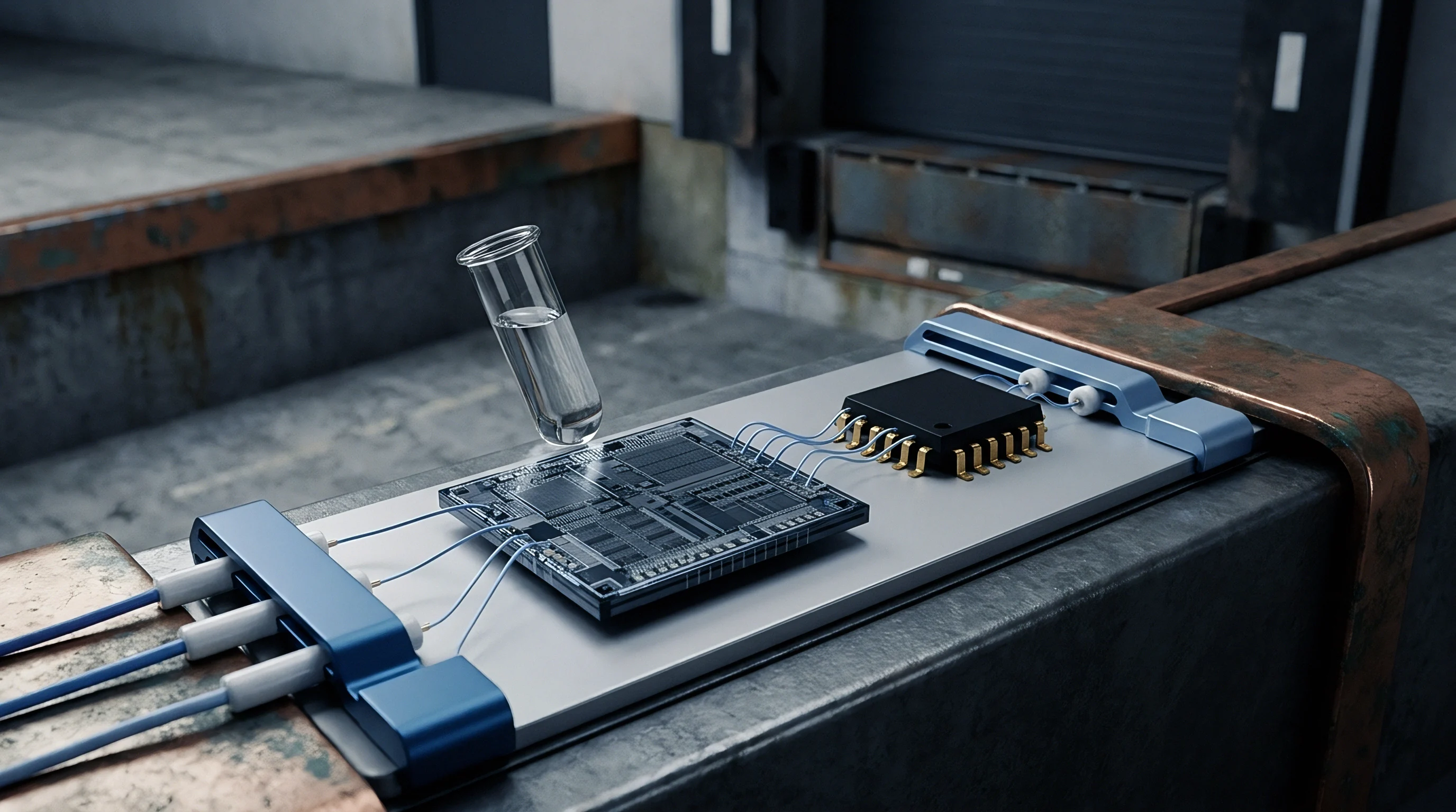
Wafer Processing and Transistor Architecture
Complementary metal-oxide semiconductor front ends achieve minimal input bias current while suffering higher low-frequency flicker transitions. Zero-drift chopper amplifiers modulate DC offset and low-frequency 1/f noise up to high switching frequencies, removing flicker noise from the operational baseband. This chopping mechanism leaves a flat white voltage noise spectral density down to direct current, making zero-drift amplifiers ideal for low-frequency precision bridge amplification.
| Amplifier Type | Voltage Noise (10 Hz) | Voltage Noise (1 kHz) | Current Noise (1 kHz) | Unit Price (1k Vol) | Lead Time (Weeks) |
|---|---|---|---|---|---|
| Ultra-Low Noise Bipolar | 1.5 nV/√Hz | 0.9 nV/√Hz | 2.2 pA/√Hz | $4.85 | 22 |
| Precision JFET Input | 8.0 nV/√Hz | 4.2 nV/√Hz | 0.005 pA/√Hz | $3.10 | 16 |
| Zero-Drift Auto-Zero | 11.0 nV/√Hz | 11.0 nV/√Hz | 0.01 pA/√Hz | $2.25 | 12 |
| General CMOS Instrumentation | 25.0 nV/√Hz | 9.0 nV/√Hz | 0.002 pA/√Hz | $0.85 | 8 |
Dual sourcing protects production. Specifying proprietary amplifier topologies without pin-compatible alternate equivalents leaves manufacturing lines vulnerable to single-source component allocation events. Sourcing teams verify that chosen package footprints align with secondary silicon vendor layouts before locking high-density printed circuit board designs.
Sole Source Risk and Qualification Cycles
Proprietary zero-drift amplifier topologies with sub-five nanovolt spectral density often originate from single semiconductor fabrication plants. Cross-qualifying alternate low-noise operational amplifiers requires validating spot noise density, input bias current temperature drift, and phase margin stability. Qualification testing cycles consume six to twelve weeks of bench characterization time and environmental chamber testing.
Zero-drift topologies chop offset. Unwanted switching clock intermodulation products generated by auto-zero amplifiers can fold back into the signal passband, introducing unexpected high-frequency spectral spikes. Sourcing agreements for low-noise front-end components enforce strict parameter limits on maximum input voltage spectral density across production batches.
Commercial procurement contracts mandate that silicon vendors maintain continuous statistical process control on low-frequency noise floors to prevent unannounced process shifts from degrading client measurement performance.
Balancing unit pricing against sole-source risk guides final silicon selection for long-lifecycle industrial instrumentation lines.