Thermal Coefficient Curvature Compensation in Precision Resistance Standard Calibration
Curvature compensation calculates temperature-dependent resistance shifts using quadratic parameters, eliminating thermal uncertainties in calibration standards.

Alloy
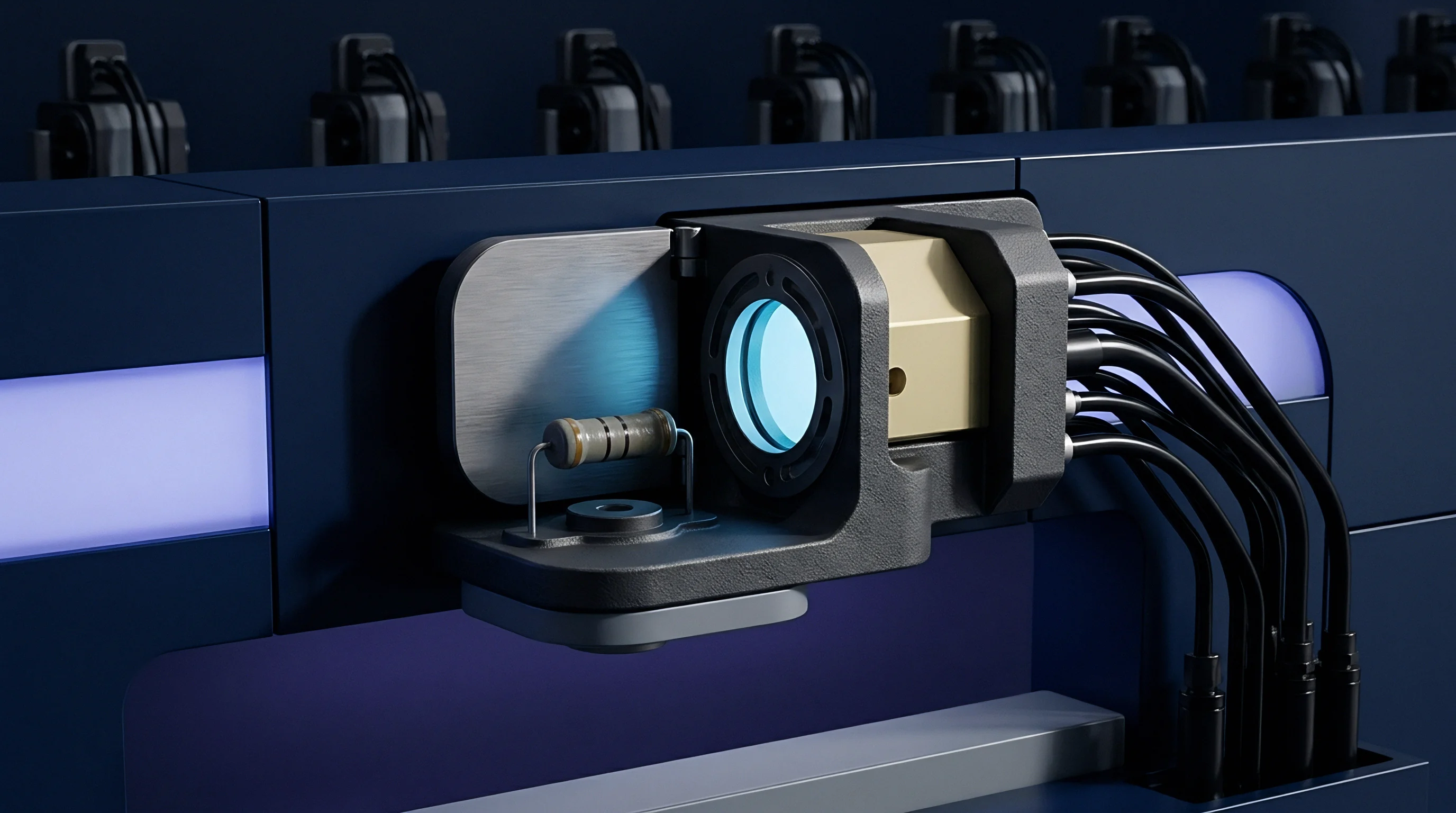
Precision resistance standards rely on solid-solution metallic alloys engineered to minimize resistivity shifts from ambient temperature changes. Primary metrology laboratories generally use standard resistors made from ternary and quaternary copper or nickel systems, such as Manganin, Evanohm, and Zeranin. Evaluating these solid-solution alloys shows that conduction behavior comes down to a balance between lattice phonon scattering and impurity scattering.
Room-temperature lattice vibrations increase resistivity linearly with temperature, while atomic disorder in the alloy matrix creates a temperature-independent baseline. By adjusting composition ratios and thermal processing, metallurgists can place a local resistivity peak or trough right inside the standard laboratory operating band, typically 20°C to 25°C.
Achieving stable performance with Manganin requires extended thermal aging.
The temperature coefficient of resistance describes how resistivity changes around a reference baseline. In standard resistors, this response is non-linear and parabolic over normal laboratory ranges. The slope near the reference temperature defines the linear coefficient (alpha), while the curve’s curvature sets the quadratic coefficient (beta).
Achieving a near-zero slope at 23°C depends on controlling atomic ordering in the lattice during wire annealing.
Solid Solution Thermodynamics and Lattice Scattering
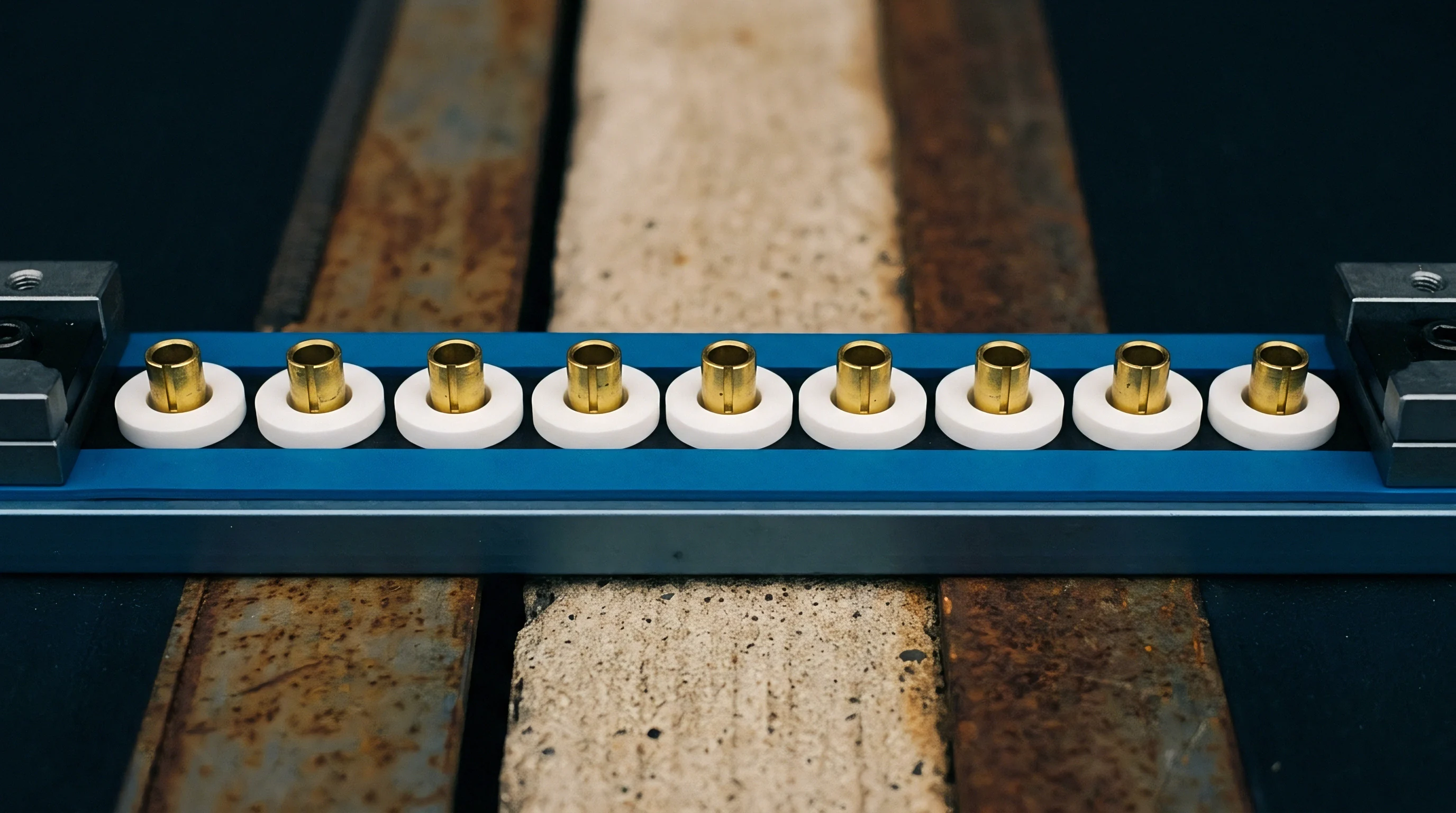
Electrical transport in precision resistive media follows the Nordheim-Gorter rule, where total resistivity is the sum of additive scattering cross-sections. In modified nickel-chromium systems containing aluminum and copper, like Evanohm, short-range atomic ordering largely controls the thermal response. Heat treatment between 400°C and 500°C induces localized atomic rearrangements that alter the conduction band and modify the density of states at the Fermi level, directly shifting the parabolic peak of the resistance-temperature curve.
Winding coils without controlling mechanical stress disrupts this lattice order. Deformation introduces dislocations that boost electron scattering, pushing alpha positive and increasing beta’s magnitude. Annealing in an inert argon atmosphere relieves strain and restores symmetry, stabilizing both coefficients.
Manufacturers then thermally age the resistors artificially to reach crystalline equilibrium before calibration mapping.
Metallurgical Factors Governing Thermal Resistance Parabola
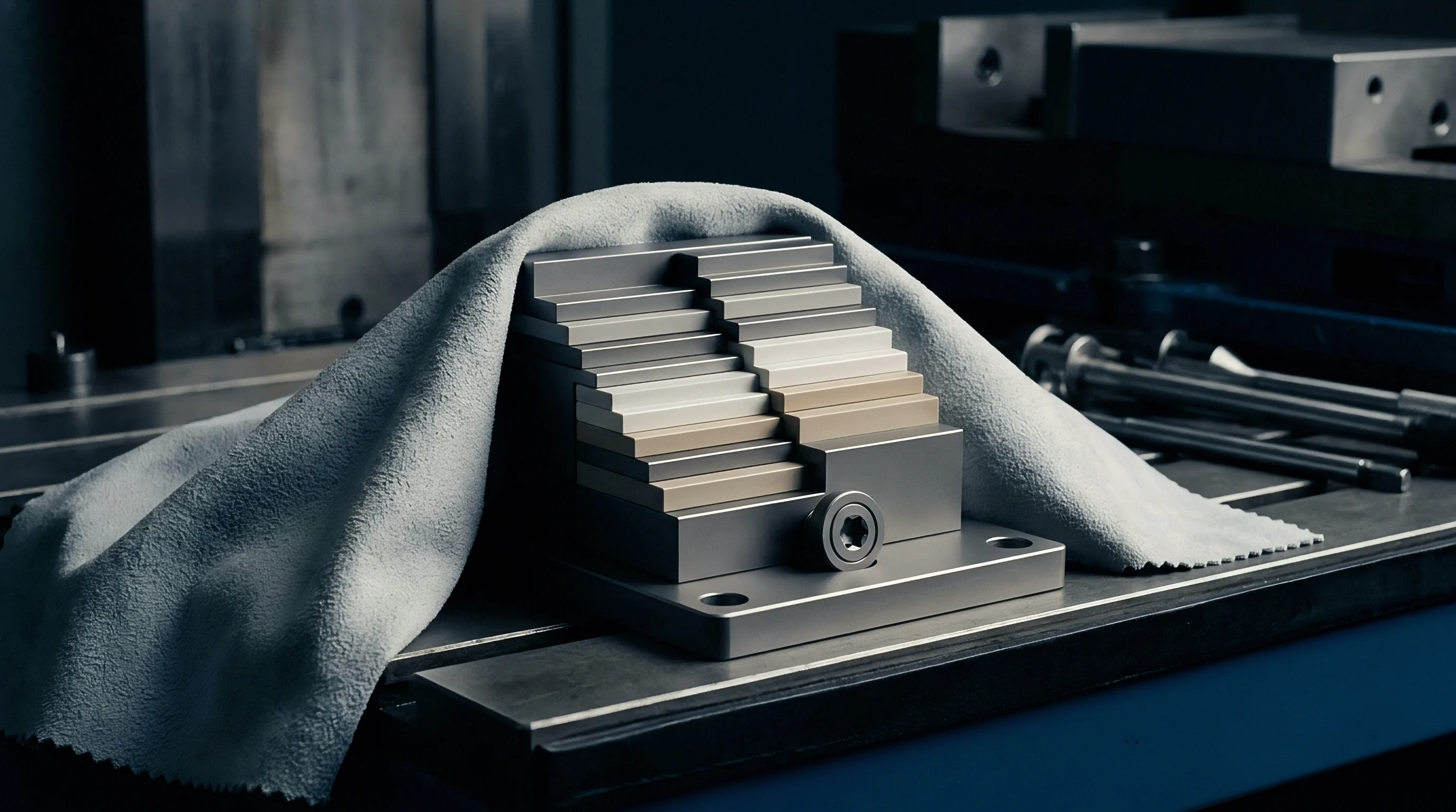
Ternary copper-manganese-nickel alloys, like Manganin, show a sharper parabolic curve than quaternary nickel-chromium systems. Because Manganin has a relatively large negative beta coefficient, its steep curve limits the uncompensated temperature window. Evanohm’s beta coefficient is nearly an order of magnitude smaller, creating a broad, flat profile ideal for sub-ppm metrology.
Zeranin sits between the two, offering reduced thermal electromotive force against copper connections.
| Alloy Composition | Nominal Alpha at 23°C (ppm/K) | Nominal Beta (ppm/K²) | Parabolic Peak Range (°C) | Thermal EMF vs Copper (µV/K) |
|---|---|---|---|---|
| Manganin (84Cu-12Mn-4Ni) | +1.5 to +15.0 | -0.35 to -0.60 | 18.0 to 26.0 | < 1.0 |
| Evanohm R (75Ni-20Cr+Al,Cu) | -1.0 to +1.0 | -0.03 to -0.06 | 20.0 to 28.0 | < 0.5 |
| Zeranin (87Cu-10Mn-3Ge) | -0.5 to +2.0 | -0.08 to -0.15 | 19.0 to 27.0 | < 0.2 |
| Karma (74Ni-20Cr-3Fe-3Al) | -2.0 to +2.0 | -0.04 to -0.08 | 21.0 to 29.0 | < 0.8 |
Choosing an alloy for a primary standard means balancing curvature, long-term drift, and parasitic thermoelectric potentials. Voltages generated at junctions introduce bias when DC polarity reversal is too slow to cancel thermal offsets. Zeranin paired with copper wiring creates very little thermoelectric noise, while Manganin junctions need strict isothermal shielding to block ambient thermal gradients.
Metallurgical degradation alters standard performance through several specific physical mechanisms:
- Solute precipitation clustering creates localized concentration imbalances in the matrix, permanently shifting the peak parabolic temperature.
- Sub-surface oxidation layer formation selectively consumes active alloy elements near wire surfaces, changing overall cross-sectional resistivity.
- Winding strain recovery relaxation changes lattice spacing over time, driving the linear coefficient alpha away from zero.
- Intermetallic phase transformation forms microscopic boundaries that increase electron scattering and alter high-temperature parabolic curvature.
Operating standard resistors outside strict isothermal baths without quadratic curvature compensation introduces unquantified errors. These flow down into secondary calibrations and invalidate reported uncertainty budgets.

Polynomial
Modeling resistance variation across temperature relies on Taylor series expansions centered on a reference temperature. In primary metrology labs, this baseline is typically set at 23.0°C or 20.0°C, depending on regional standards. A quadratic expansion tracks actual physical curve behavior accurately over narrow temperature spans, while extending the expansion to cubic terms captures distortion that emerges across wider temperature characterizations.
Crystalline structures show a symmetrical parabolic response near their turning point temperature. The second-order expansion relates measured resistance to baseline resistance through linear alpha and quadratic beta terms:
R(T) = R_ref
Higher-order thermal effects introduce slight asymmetries into this parabola. Standard calibration certificates state alpha and beta derived from least-squares fitting across stabilized temperature points. Over wider temperature ranges, a cubic gamma coefficient is added to account for asymmetry in electron scattering.

Mathematical Formulations for Resistance Temperature Dependence
Evaluating resistor behavior during ambient shifts requires finding the turning point temperature ~ the point where the temperature derivative of resistance equals zero. Differentiating the quadratic equation gives the peak temperature:
T_peak = T_ref – (alpha / (2 beta))
When alpha is zero, the turning point hits the reference temperature exactly, making resistance insensitive to small thermal fluctuations. Metallurgical heat treatment aims to align T_peak with standard lab operating temperatures. If a resistor has a positive alpha at 23°C, its turning point lies above 23°C, so resistance increases as temperature rises toward T_peak.
Past T_peak, the negative beta coefficient takes over, pulling resistance down as temperature continues to rise.
Cubic compensation terms reduce residual interpolation errors below 0.02 parts per million when calibrating Evanohm resistance standards across a 15°C to 30°C thermal range.
Evanohm exhibits exceptionally low linear drift over extended periods.
Adjusting precision standards uses controlled heat treatment to drive alpha to zero. Beta, however, is an intrinsic alloy property that barely responds to heat treatment variations. Curvature compensation software remains necessary for accurate measurements whenever ambient room temperatures fluctuate.
Residual Errors in Lower Order Expansions
Truncating the model to a linear approximation introduces significant systematic error. Even in controlled rooms held within 23.0°C ± 0.5°C, uncompensated quadratic curvature causes measurable errors in high-accuracy standards.
| Ambient Offset from Reference (K) | Linear-Only Model Residual (ppm) | Parabolic Quadratic Residual (ppm) | Cubic Expanded Residual (ppm) | Uncompensated Drift Deviation (µΩ) |
|---|---|---|---|---|
| ± 0.5 | 0.25 | 0.008 | 0.001 | 80 |
| ± 1.0 | 0.50 | 0.032 | 0.002 | 320 |
| ± 2.0 | 1.00 | 0.128 | 0.005 | 1280 |
| ± 5.0 | 2.50 | 0.800 | 0.022 | 8000 |
Cubic models become necessary when calibration uncertainty must stay below 0.05 ppm across broader temperature spans. As shown in the table above, parabolic models capture over 98% of thermal resistance variation within ± 2.0°C of reference equilibrium, but cubic terms are needed to eliminate systematic bias further out.
Higher-order lattice vibrational modes can also affect quadratic coefficient stability during rapid ambient temperature transitions.

Bath
Bench calibrations require precise thermal control systems that keep spatial gradients below 2 millikelvin throughout the working volume. Mapping precision resistors relies on circulating mineral oil baths, temperature-controlled air enclosures, or solid-state Peltier systems. Liquid immersion provides superior heat transfer, rapidly dampening internal thermal oscillations and carrying away self-heating generated by test currents.
Fluid circulation in oil baths maintains tight spatial thermal equilibrium throughout the bath volume.
When isolating self-heating in an oil bath, heat moving from the resistive element through its internal insulation into the bath fluid sets up a temperature gradient. The wire core operates warmer than the bath’s temperature sensor. Characterizing curvature accurately requires separating ambient fluid temperature shifts from electrical self-heating.

Thermal Gradient Limits Affecting Curvature Mapping Accuracy
Spatial gradients across an oil bath introduce systematic calibration bias. If the reference thermometer sits 10 centimeters from the resistor body in a bath with a 10 millikelvin gradient, the fitted thermal model absorbs an artificial temperature offset. Motor dissipation, fluid velocity, and insulation geometry ultimately set the bath’s spatial uniformity limits.
Standard Platinum Resistance Thermometers (SPRTs) placed next to resistor housings provide primary temperature tracking. Measurement bridges record thermometric resistance alongside standard resistor ratios, linking applied thermal states directly to resistance values. Bath control instability beyond 1 millikelvin introduces scatter that degrades quadratic curve fits.
Standard ISO 17025 accredited calibration protocols require spatial bath thermal uniformity better than 0.003°C to achieve standard resistor alpha parameter mapping uncertainties under 0.05 ppm/K.
Dissipation Power Corrections and Extrapolation Methods
Measuring resistance requires passing a current, which dissipates thermal power in the resistor via Joule heating (P = I^2 R). This internal power raises the element’s temperature above the surrounding fluid. The power dissipation coefficient ~ expressed in milliwatts per kelvin or ppm per milliwatt ~ quantifies thermal resistance through the potting compound and enclosure.
Zero-power extrapolation mathematically isolates and removes these self-heating errors.
Finding true resistance at zero applied power requires measuring resistance at two excitation currents, typically I and I sqrt(2), which corresponds to a 1:2 power ratio. The standard zero-power extrapolation steps are:
- Stabilize the thermal bath at the target calibration temperature point within 1 millikelvin limits for at least 120 minutes.
- Apply the primary measurement current I_1 to the standard resistor and record resistance equilibrium once thermal dissipation achieves steady state.
- Increase the measurement current to I_2 = I_1 1.414, doubling the internal power dissipation without altering bath temperature settings.
- Record the elevated resistance value R_2 after internal heat dissipation achieves thermal equilibrium within the resistor housing.
- Calculate the self-heating power coefficient theta using the resistance differential divided by applied power variation delta P.
- Subtract the product of theta and base power P_1 from measured resistance R_1 to compute the zero-power resistance state R_zero.
- Repeat the zero-power calculation across every calibration temperature node prior to fitting the quadratic coefficient matrix.
Internal heat sinks do not eliminate power dissipation errors entirely; precision measurements show internal temperature rises persist regardless of housing design.

Arithmetic
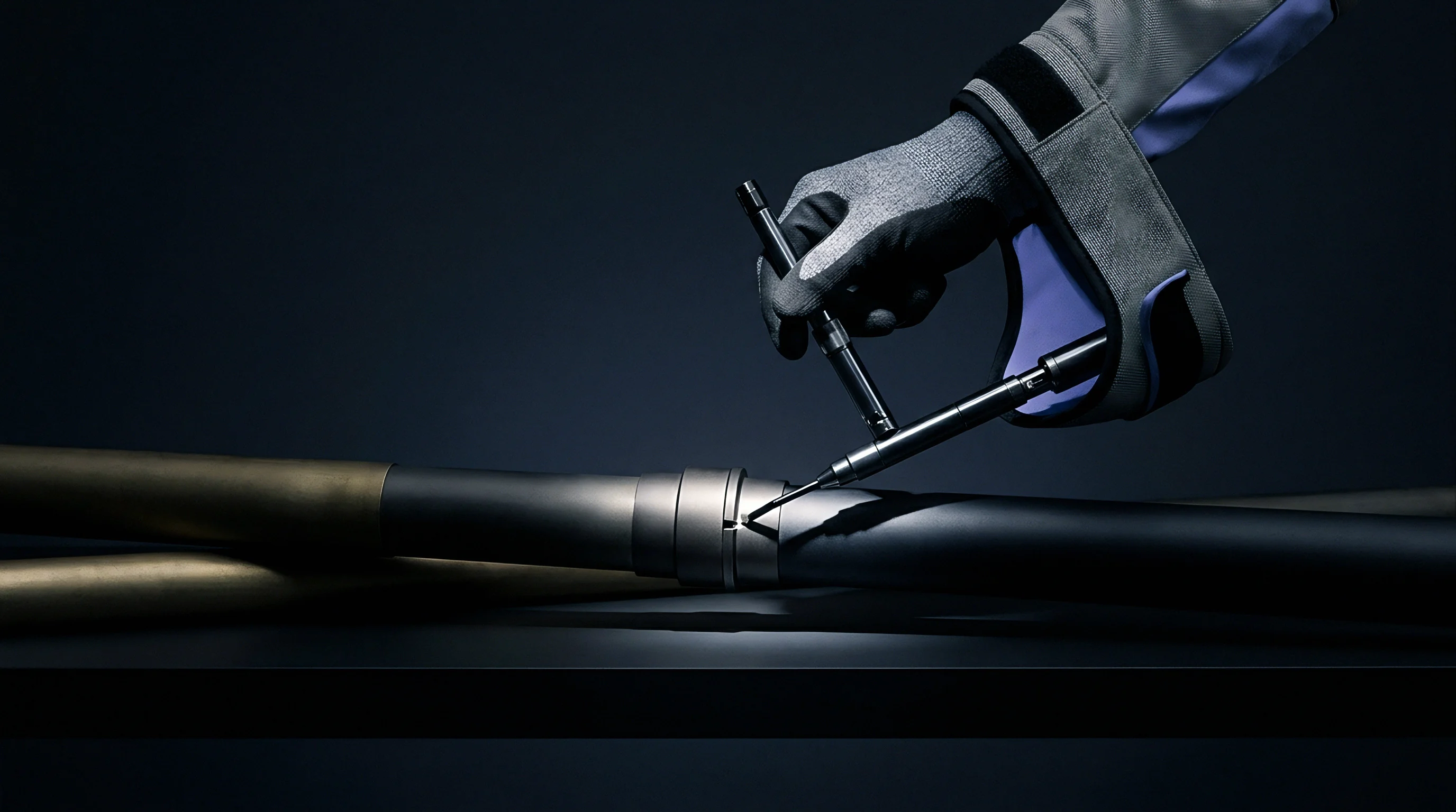
Calculating alpha and beta coefficients relies on linear regression applied to multi-point temperature-resistance data. Calibration protocols record resistance at five or more stabilized temperatures spanning the operating range. When computing the least-squares normal equations, matrix formulation avoids numerical instability and spreads residual measurement noise evenly across the extracted parameters.
Non-linear thermal curvature requires extending the correction matrix beyond linear terms.
Let vector Y represent fractional resistance deviations from nominal, and matrix X hold the thermal offset terms. The design matrix has columns for the unit baseline, linear temperature offset (T – T_ref), and quadratic offset (T – T_ref)^2. Inverting and multiplying yields the parameter vector containing baseline shift, alpha, and beta.

Least Squares Regression Matrix for Parameter Extraction
Constructing design matrix X for temperature test points T = °C with T_ref = 23.0°C requires evaluating offset powers. The offset vector dt = K forms the second column, and squared offsets dt^2 = K² form the third. Matrix multiplication X^T X produces a symmetric 3×3 normal matrix:
X^T X =
Choosing symmetric test points around T_ref simplifies computation by pushing odd power sums, sum(dt) and sum(dt^3), to zero. This orthogonality uncouples baseline resistance and quadratic beta calculations from linear alpha estimation, reducing parameter covariance and suppressing error propagation during matrix inversion.
Evaluating the matrix residual norm confirms the statistical validity of the polynomial fit.
Solving (X^T X)^(-1) X^T Y calculates each thermal parameter along with its standard error. Evaluating residual variance confirms whether a parabolic model fits observed behavior or if third-order terms are necessary.
Propagation of Thermometric Measurement Errors
Uncertainties in reference thermometry convert directly into parameter uncertainties. Temperature noise widens parameter covariance bounds proportional to derivative sensitivity factors.
| Uncertainty Component Source | Standard Uncertainty Value | Probability Distribution Type | Sensitivity Coefficient | Uncertainty Contribution (ppm) |
|---|---|---|---|---|
| SPRT Calibration Reference | 0.0015 K | Normal (k = 2) | alpha = 0.05 ppm/K | 0.000075 |
| Bath Spatial Gradient Uniformity | 0.0020 K | Rectangular | alpha = 0.05 ppm/K | 0.000058 |
| DC Comparator Bridge Ratio Non-linearity | 0.015 ppm | Normal (k = 1) | 1.0 | 0.015000 |
| Self-Heating Power Extrapolation | 0.005 ppm | Rectangular | 1.0 | 0.002887 |
| Polynomial Regression Residual Fit | 0.008 ppm | Normal (k = 1) | 1.0 | 0.008000 |
Calculating total uncertainty requires combining individual variance contributions in quadrature per ISO Guide to the Expression of Uncertainty in Measurement (GUM) guidelines. Decoupled symmetric temperature steps suppress covariance cross-terms, simplifying combined standard uncertainty calculations.
Calibrating standard resistors using symmetric temperature arrays around 23.0°C eliminates covariance cross-terms between linear alpha and quadratic beta fitting parameters.
Validating extracted curvature parameters against historical calibration records involves several key checks:
- Thermal parameter sign verification confirms negative beta values consistent with solid-solution parabolic resistance physics.
- Turning point peak check calculates T_peak to confirm the parabolic peak stays within standard laboratory operating limits.
- Residual variance ratio test verifies that residual errors are randomly distributed within Chi-squared confidence limits.
- Covariance matrix magnitude audit checks off-diagonal covariance terms to verify that thermal node symmetry uncoupled the model parameters.
Calculating mathematical corrections without incorporating temperature measurement uncertainties leads to unrealistically optimistic uncertainty budgets that will not survive peer review.


Relaxation
Long-term drift in precision standards stems from atomic rearrangement, stress relaxation, and oxidation within the element. As baseline resistance shifts over time, thermal coefficient parameters gradually drift as well. Tracking standard resistors over multi-year recalibration cycles shows that structural relaxation alters internal strain distributions ~ shifting alpha while beta stays relatively constant.
Gradual strain relief within the alloy wire remains the primary driver of long-term drift.
Temperature spikes during transport or storage speed up atomic migration, disrupting carefully stabilized thermal profiles. Resistors exposed to thermal extremes outside design limits develop microstructural dislocations that alter resistivity, requiring a complete re-mapping of their temperature coefficients.
Microstructural Aging Mechanisms in Precision Wire
Solid-state diffusion in nickel-chromium and copper-manganese alloys causes vacancy annihilation and short-range reordering. In Evanohm wire, low-temperature heat treatments set up specific atomic configurations that optimize stability. Over years at 23°C ambient temperatures, residual thermodynamic forces maintain slow atomic diffusion toward equilibrium.
Junctions between internal alloy wire and copper terminal leads generate small parasitic thermal electromotive forces.
Vacancy migration changes electron mean free path distributions, shifting baseline resistance R_0 and subtly altering alpha. Micro-strain relief lowers local stress concentrations, gradually nudging alpha in a negative direction over extended operating lifetimes.
Thermal Cycling Hysteresis and Permanent Resistance Offsets
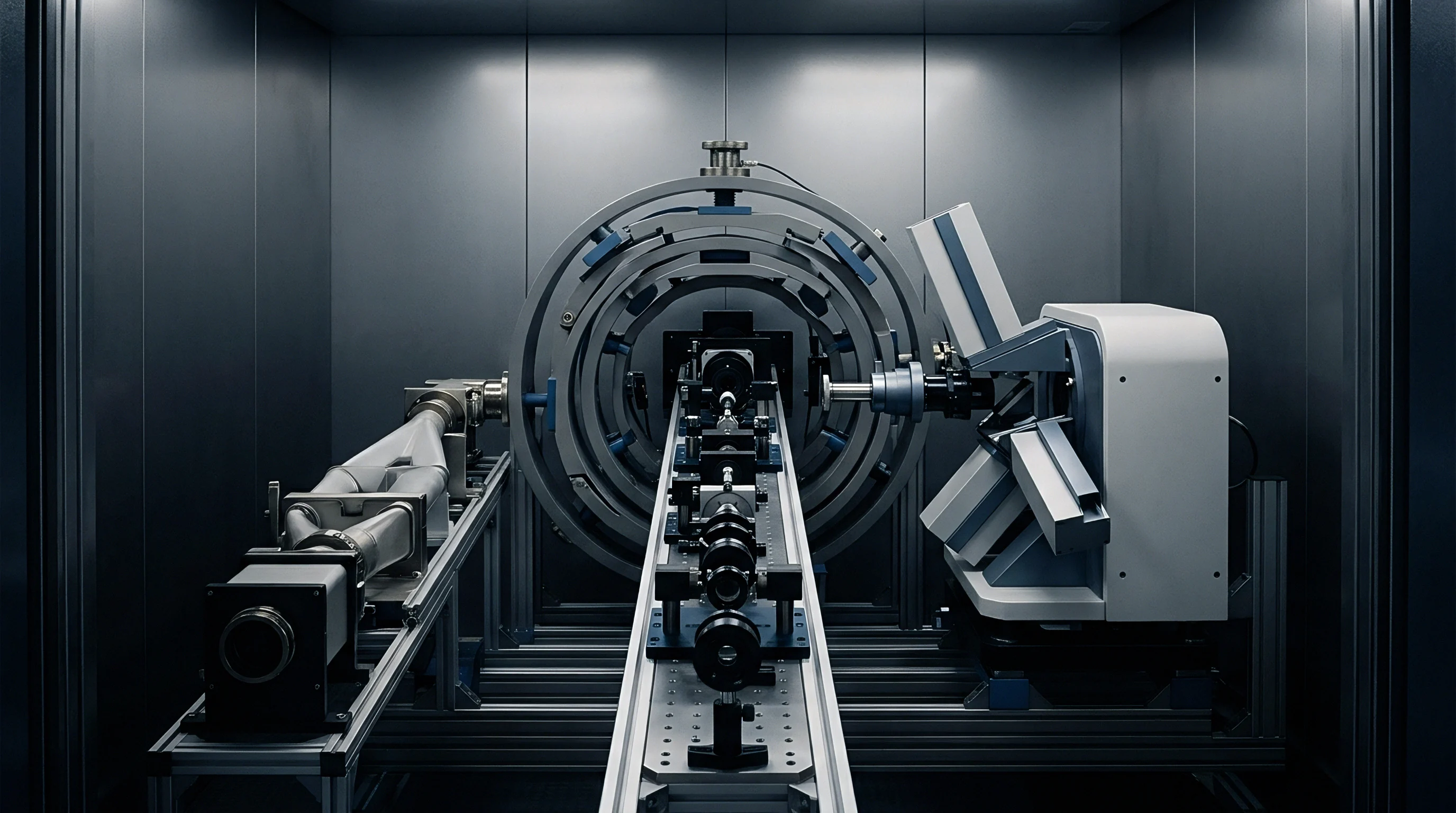
Cycling resistors between operational and storage temperature extremes creates thermal expansion mismatch stresses between the alloy wire, support bobbins, and encapsulation compound. This mechanical stress causes plastic deformation in the wire, altering crystal symmetry.
Thermal excursions exceeding 40°C introduce irreversible strain-induced offsets in Manganin resistance standards, altering baseline values by up to 0.5 ppm.
Thermal hysteresis shows up as residual resistance offsets when the standard returns to reference temperature. Resistors with noticeable hysteresis require extended settling periods ~ from weeks to months ~ to re-establish mechanical equilibrium before high-accuracy calibration.
Severe thermal hysteresis leads to permanent baseline offsets that cannot be recovered through thermal stabilization alone.
Auditing routines track coefficient stability to separate alloy drift from surface oxidation. Metrology leads use the following criteria to schedule re-characterization intervals:
- Multi-year alpha tracking trend analysis identifies linear coefficient drift trends exceeding twice the published calibration uncertainty bounds.
- Post-transit verification mapping checks baseline resistance stability after shipment between international calibration facilities.
- Self-heating coefficient stability audits detect potential degradation in the internal thermal potting compound’s conductivity.
- Thermal hysteresis loop quantification measures residual resistance offsets following deliberate ±5°C thermal cycling excursions.
As a rule of thumb, any standard resistor subjected to an unmonitored temperature excursion past 50°C must undergo complete multi-point re-characterization before returning to primary calibration service.

Docket
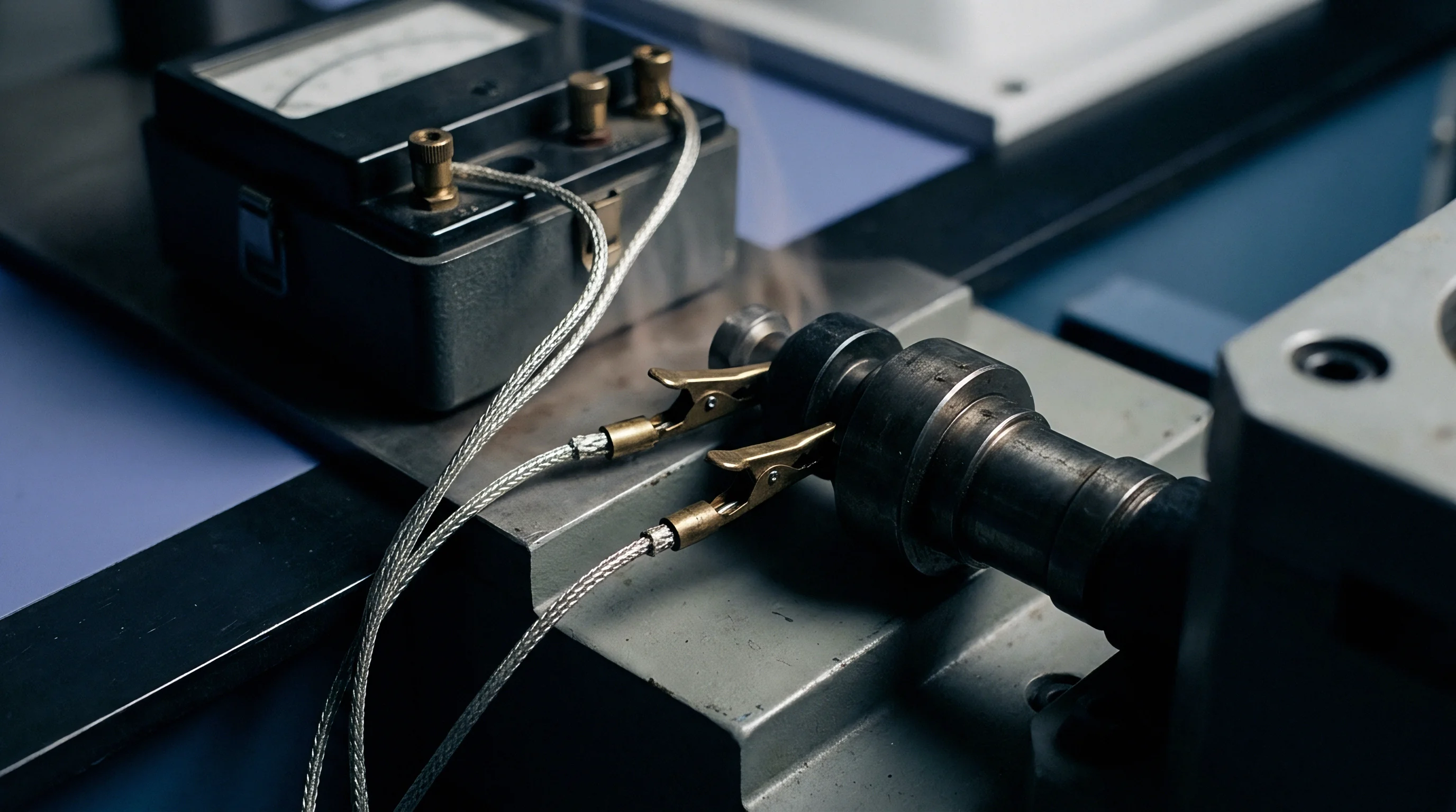
Procuring precision resistance standards and contracting accredited calibration requires explicit specifications for temperature coefficient characterization. Standard commercial calibration certificates often report resistance at a single temperature, omitting thermal curvature parameters unless specifically required by contract. Buyers reviewing vendor scope documents must verify accredited mapping ranges and thermometric measurement uncertainty limits.
Maintaining primary precision standards requires rigorous characterization across the full operating thermal range.
Uncertainty statements on calibration certificates carry defined environmental boundaries. Using standard resistors outside accredited ambient temperature ranges without applying verified curvature compensation breaks the traceable measurement chain to national metrology institutes.
Scope Verification for ISO Seventeen Twenty Five Calibration Laboratories
Accreditation scopes published under ISO/IEC 17025 detail Calibration and Measurement Capabilities (CMC) across specific parameter fields. Metrology managers reviewing vendor scopes must confirm that accreditation explicitly covers multi-point thermal mapping rather than simple single-point checks.
Calibration certificates document the exact reference conditions under which uncertainties remain valid.
Uncertainty budgets published by accredited labs combine reference thermometry uncertainty, bath gradient limits, bridge ratio errors, and residual regression variance. Procurement specifications should mandate reporting full matrix covariance parameters along with alpha, beta, and baseline resistance values to ensure compatibility with automated compensation software.

Commercial Economics of Mapped Temperature Standards
Sourcing fully characterized primary standards carries higher initial costs but reduces long-term measurement risk. Resistors operating in air without oil bath stabilization experience room fluctuations up to ±2°C. Using uncompensated standards across varying room temperatures adds unquantified systematic uncertainty that degrades secondary calibration margins.
Uncertainty budgets expand significantly near the boundaries of specified thermal operating windows.
Procurement contracts should include explicit acceptance clauses requiring vendors to supply verified multi-point temperature coefficient datasets recorded across five or more stabilized thermal nodes, certified under ISO/IEC 17025 with expanded uncertainty bounds stated for all extracted polynomial parameters.