Quantifying Uncorrected Thermal Gradient Uncertainty Contributions in Distributed High Precision Sensor Calibration Infrastructure
Uncorrected manifold thermal gradients inflate calibration uncertainty, forcing tight guardbands that spike manufacturing scrap and compromise traceable sensor accuracy.
Fluke
Distributed calibration manifolds exhibit spatial thermal non-uniformities that evade single-point reference probes. A primary standard reading 25.000 degrees Celsius across a central well guarantees nothing about the boundary temperature four ports away. In automated test racks operating twenty-four ports simultaneously, spatial differences routinely reach 45 millikelvin.
That divergence compromises Class AA resistance thermometers before factoring in lead resistance or instrumentation noise.
Buyers routinely discover this disparity during third-party site audits. A manifold certified to 8 millikelvin expanded uncertainty within an isolated liquid bath drifts to 60 millikelvin when populated with active sensor wiring harnesses. Conduction down copper leads pulls local sensor wells toward ambient factory conditions.
The primary standard remains thermally isolated within its deep thermowell, recording an undisturbed baseline while adjacent positions wander.
Uncorrected gradients enter the uncertainty budget through spatial non-uniformity, temporal stability drift, and dynamic thermal immersion deficits. Metrologists characterize spatial gradients via multi-point differential arrays according to Euramet guidelines. The baseline uncertainty balance establishes the initial baseline for manifold qualification:
The total spatial uncertainty contribution matches the root sum square of orthogonal components. Radial gradients, axial immersion gradients, and port-to-port azimuthal differences compound concurrently:
u_spatial = sqrt( u_radial^2 + u_axial^2 + u_azimuthal^2 )
Calibrating miniature platinum resistance elements without verifying local port immersion introduces gross errors. Industrial thermowells often feature shallow insertion depths below five sensing lengths. Conduction losses down the sheath generate systematic offsets exceeding the entire tolerance band of the device under test.
A commercial calibration certificate remains valid only within the specific immersion depth and thermal boundary conditions verified during laboratory qualification.
The standard testing procedure assumes equilibrium across all test positions. Real-world manifolds rarely achieve steady-state conditions during high-throughput cycling. Air currents across external sensor wiring establish persistent thermal shunts.
These shunts distort the local heat flux field inside equalizing blocks, shifting apparent sensor calibration points away from true bath values.
The section leaves open whether dynamic numerical modeling can replace dense sensor physical arrays when characterizing irregular geometric manifolds under high fluid velocity.
Draft
Air movement inside testing chambers generates localized convective variations across passive sensor arrays. Calibration fixtures rely heavily on forced convection to maintain setpoint stability, yet turbulent boundary layer separation induces localized temperature depressions. A 2 meter per second localized draft across an uninsulated terminal block drops its temperature by 180 millikelvin relative to an adjacent shielded channel.
These boundary disturbances penetrate deep into standard thermowells through metallic conduction paths. Copper leads, thin-walled stainless steel sheaths, and brass compression fittings act as heat pipes between ambient air and internal sensor elements. Minimizing this effect requires insulating outer fixtures or actively controlling dry-well zone heaters.
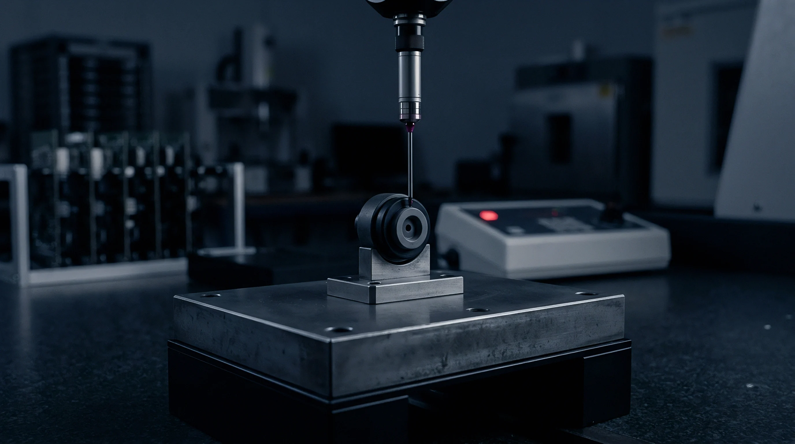
Convection Boundary Layer Disturbances
Forced convection inside environmental testing chambers rarely produces laminar conditions across sensor trees. Recirculation fans induce chaotic velocity vectors, yielding Nusselt numbers that vary by 35 percent across a 300-millimeter horizontal span. Local convective heat transfer coefficients swing between 25 and 65 watts per square meter Kelvin.
The resulting variation in stem conduction losses directly skews sensor readings.
Insulation collars mitigate external convective coupling. Ceramic fiber wraps and closed-cell elastomeric foams isolate fixture top plates from ambient chamber drafts. Without protective lagging, ambient drafts create a persistent 12 millikelvin gradient between peripheral ports and the central reference well.
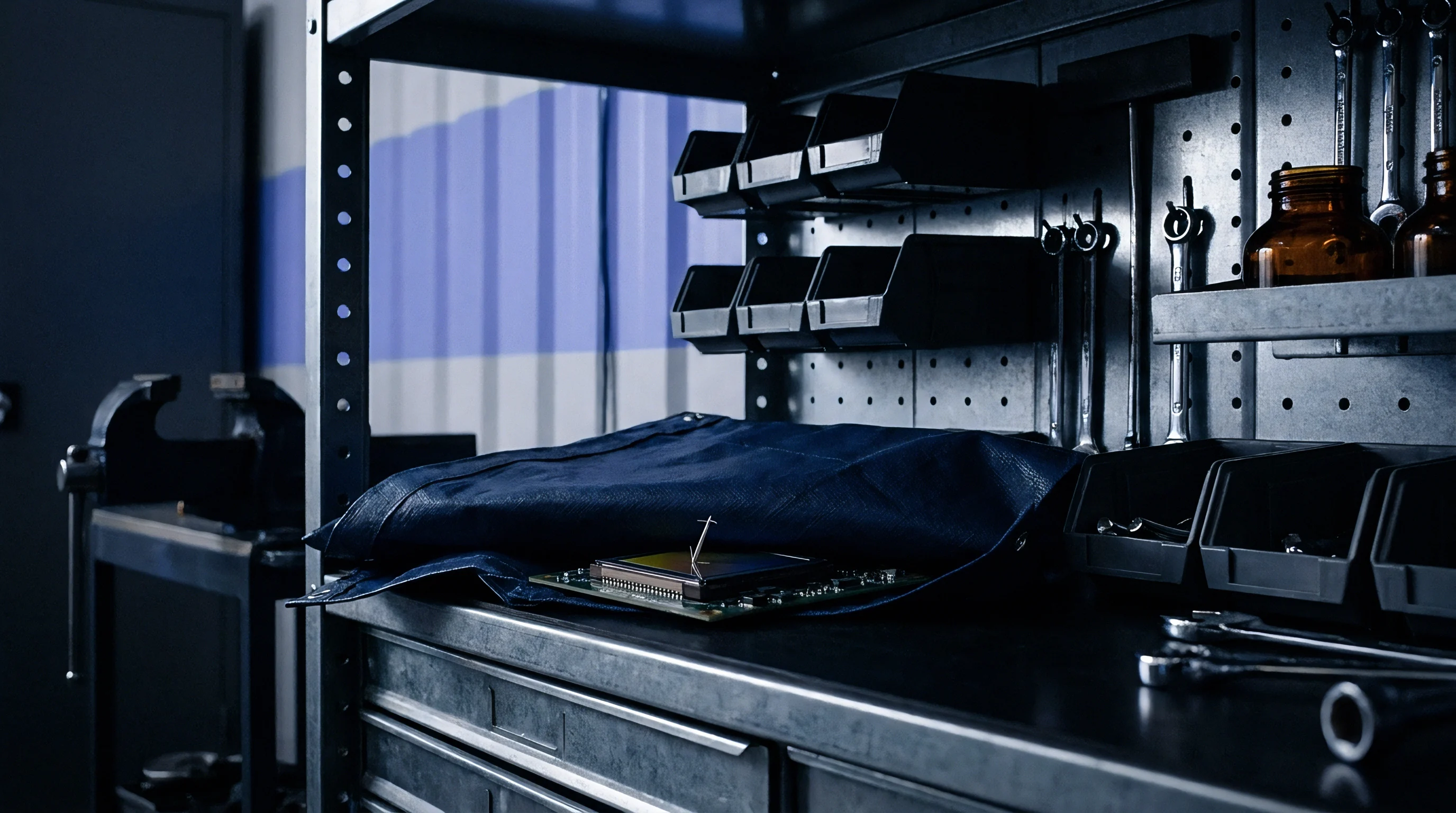
Conduction Shunts along Wiring Looms
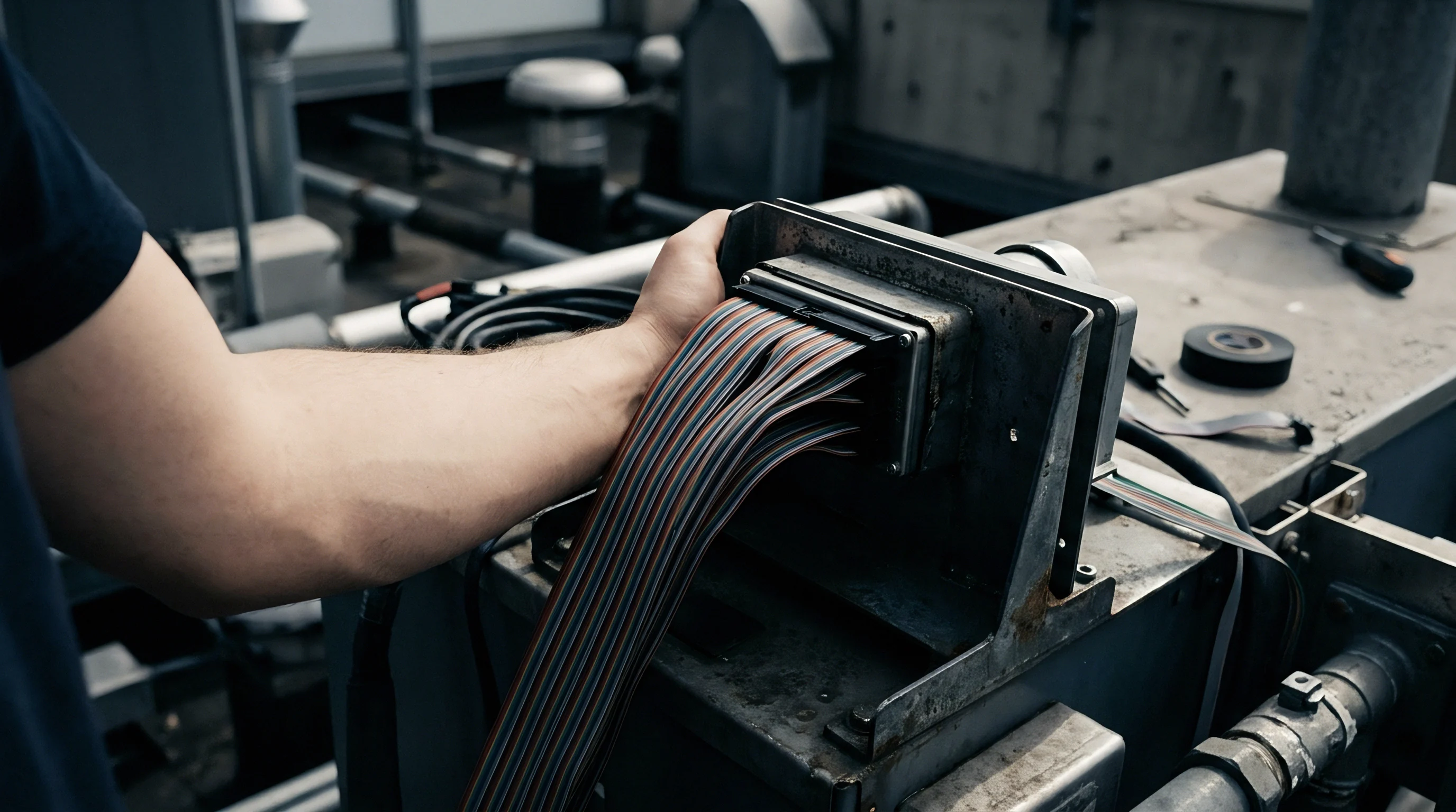
Cables bundle thermal conduction paths directly to sensor elements. A 24-core measurement cable containing 24 AWG copper conductors acts as a low-resistance path for ambient thermal infiltration. Each copper core features thermal conductivity exceeding 380 watts per meter Kelvin, routing heat outward during hot calibrations and inward during cryostat runs.
Standard four-wire RTD configurations eliminate electrical lead resistance errors while leaving thermal conduction shunts unmitigated. The sensing element assumes a hybrid temperature between the calibration core and external terminal block. Mitigating this error involves heat-sinking incoming wires to equalizing blocks prior to entering sensing cavities.
| Conductor Material | Cross-Section (mm²) | Immersion Depth (mm) | Uncorrected Offset (mK) | Standard Uncertainty (mK) |
|---|---|---|---|---|
| Solid Copper 24 AWG | 0.205 | 80 | 38.4 | 11.1 |
| Stranded Copper 26 AWG | 0.128 | 80 | 24.2 | 7.0 |
| Solid Nickel 24 AWG | 0.205 | 80 | 9.1 | 2.6 |
| Solid Copper 24 AWG | 0.205 | 160 | 2.1 | 0.6 |
| Constantan 24 AWG | 0.205 | 80 | 2.3 | 0.7 |
Stem conduction errors scale exponentially with immersion depth. Doubling sensor immersion depth from 80 to 160 millimeters reduces the thermal conduction offset from 38.4 millikelvin down to 2.1 millikelvin under identical airflow conditions. Calibrators frequently compromise immersion depths when testing high-density sensor batches, introducing significant uncorrected thermal errors.
Ignoring external airflow patterns and wiring thermal sinking transforms a precision calibration procedure into an uncontrolled indicator of room air velocity.
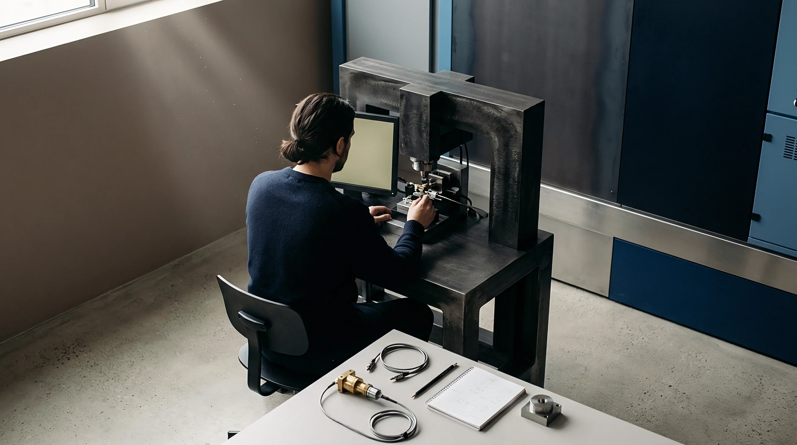
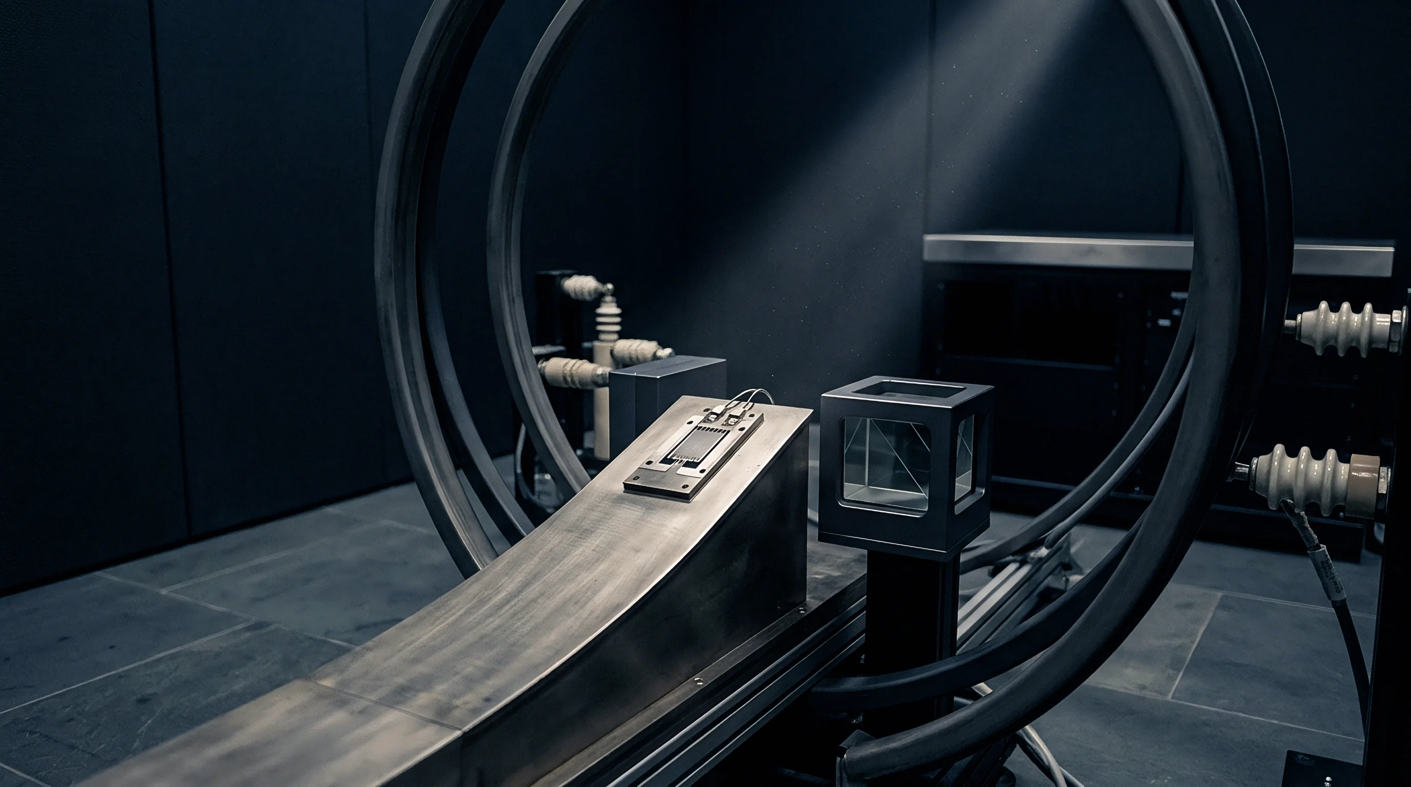
Block
Solid metal equalizing inserts serve as the core thermal reservoir for multi-well dry blocks. Material selection governs the internal temperature distribution. Oxygen-free high-conductivity copper provides exceptional thermal performance near room temperature, while nickel-plated aluminum alloys dominate commercial multi-well inserts due to weight and machining economics.
Alloy selection alters internal spatial performance significantly. Aluminum 6061-T6 displays a thermal conductivity around 167 watts per meter Kelvin at 20 degrees Celsius. In contrast, copper 101 exhibits 391 watts per meter Kelvin.
Under a 5-watt parasitic heat loss down a sensor sheath, an aluminum block develops an internal localized gradient more than double that of a copper equivalent.

Radial and Axial Flux Imbalance
Cartridge heaters embedded along dry-block walls generate discrete radial flux vectors. Because heaters cannot deliver continuous, uniform thermal flux, heat flows through discrete conduction pathways into the central mass. Azimuthal temperature variations emerge across symmetrically arranged peripheral test wells.
Axial temperature profiles present severe challenges across deep calibration zones. Dry blocks feature base heaters and top guard heaters designed to establish an isothermal zone. Mismatched tuning between upper and lower control zones creates a parabolic temperature profile along the insert axis.
An insertion depth shift of 5 millimeters introduces up to 18 millikelvin of bias into platinum resistance thermometer calibrations.
- Immersion depth verification ensures the sensing element resides entirely inside the characterized uniform zone of the insert block.
- Well clearance profiling prevents air insulation gaps from creating unpredictable radial thermal drop between metal insert walls and sensor sheaths.
- Radial symmetry mapping identifies port-to-port temperature offsets across symmetrically machined boreholes under operational thermal loads.
- Thermal compound application bridges air gaps within wells to suppress contact resistance variations across high-throughput production runs.
Air gaps between the sensor sheath and insert well bore introduce thermal contact resistances exceeding 0.05 meters squared Kelvin per watt. In dry calibration systems without heat transfer fluids, an off-center sensor experiences severe azimuthal asymmetry. Heat flows through direct contact points while stalling across static air gaps, yielding inconsistent calibrations across repeated insertions.
Liquid calibration baths mitigate contact resistance issues but introduce fluid dynamic circulation complexities. Fluid velocity variances across impeller-driven baths establish pressure and boundary layer variations against sensor sheaths. Pockets of stagnant fluid inside dense sensor racks generate thermal dead zones that degrade measurement accuracy.
A metal block insert acts as an averaging filter for rapid temporal heater oscillations while preserving static spatial temperature gradients across its boreholes.
A supplier often claims that equalizing inserts display zero internal temperature differences because finite element models assume perfectly insulated boundary surfaces.
Math
Building an uncertainty budget for distributed sensor calibration requires quantifying each spatial and temporal gradient contribution under the JCGM 100:2008 Guide to the Expression of Uncertainty in Measurement. Spatial variances cannot simply be averaged out; they represent systematic boundary offsets with rectangular or U-shaped probability distributions. Metrologists must calculate these uncertainties across radial, axial, and temporal dimensions to prevent systematic errors.
Consider a 16-port distributed calibration manifold testing Class A thin-film Pt100 elements at 150.00 degrees Celsius. The central well houses a certified standard platinum resistance thermometer. Peripheral wells contain industrial probes connected via uninsulated leads.
The laboratory measures the maximum radial difference across all outer ports at 32 millikelvin. The axial profile over a 30-millimeter vertical span shows a 14 millikelvin drift, while temporal stability across a 30-minute test cycle demonstrates a 6 millikelvin peak-to-peak oscillation.
Probability Distribution Assignments
Radial temperature variations across symmetric wells follow rectangular probability distributions. Without continuous multi-channel thermometry across every well, any temperature within the measured envelope remains equally probable. The radial standard uncertainty calculates as the half-width divided by the square root of three:
u_rad = 0.032 / (2 sqrt(3)) = 0.00924 K
Axial immersion variations follow asymmetric triangular distributions when insertion depths are mechanically fixed against an insert base. When sensor positioning fluctuates within a tolerance band, a rectangular distribution applies across the displacement span:
u_ax = 0.014 / (2 sqrt(3)) = 0.00404 K
Temporal stability reflects sinusoidal oscillations driven by proportional-integral-derivative heater loops. This periodic behavior produces a U-shaped probability distribution with significant time spent at upper and lower turning points:
u_temp = 0.006 / (2 sqrt(2)) = 0.00212 K
Combined Budget Synthesis
Thermal gradients also induce parasitic thermoelectric voltages along sensor wiring harnesses. Dissimilar metals exposed to internal temperature gradients generate microvolt-level Seebeck offsets. For resistance measurements using direct-current excitation, these voltages create apparent resistance shifts.
The metrologist must incorporate this parameter into the combined budget alongside standard physical temperature gradients.
| Uncertainty Component | Value (mK) | Probability Distribution | Divisor | Standard Uncertainty u_i (mK) | Sensitivity Coefficient c_i | Contribution u_i c_i (mK) |
|---|---|---|---|---|---|---|
| Reference Standard Calibration | 4.50 | Normal (k=2) | 2.000 | 2.25 | 1.0 | 2.25 |
| Radial Well-to-Well Non-Uniformity | 32.00 | Rectangular | 3.464 | 9.24 | 1.0 | 9.24 |
| Axial Thermal Gradient | 14.00 | Rectangular | 3.464 | 4.04 | 1.0 | 4.04 |
| Temporal Temperature Stability | 6.00 | U-Shaped | 2.828 | 2.12 | 1.0 | 2.12 |
| Stem Conduction Parasitic Loss | 18.50 | Rectangular | 3.464 | 5.34 | 1.0 | 5.34 |
| Parasitic Seebeck Thermal EMF | 3.20 | Rectangular | 3.464 | 0.92 | 1.0 | 0.92 |
| Contact Resistance Variability | 8.00 | Rectangular | 3.464 | 2.31 | 1.0 | 2.31 |
Summing these components via root sum square yields the combined standard uncertainty for the distributed calibration infrastructure:
u_c = sqrt( 2.25^2 + 9.24^2 + 4.04^2 + 2.12^2 + 5.34^2 + 0.92^2 + 2.31^2 ) = 12.35 mK
Applying a coverage factor of k = 2 for an approximate 95 percent level of confidence expands the calibration uncertainty to 24.70 millikelvin. Radial non-uniformity dominates this uncertainty budget, contributing over half of the total variance. In contrast, the calibrated primary reference probe contributes a modest fraction to the combined result.
u_c = 12.35 mK represents the baseline calibration floor for the 16-port manifold under steady-state operating conditions at 150 degrees Celsius.
Omitting spatial non-uniformity terms produces artificially low uncertainty claims that fail standard accreditation audits and cause out-of-tolerance sensor returns from downstream clients.

Drift
Thermal gradients rarely remain static over extended calibration campaigns. Heating element degradation, oxidation along dry-block insert interfaces, and settling insulation create time-dependent gradient growth. A calibration manifold exhibiting balanced 10 millikelvin uniformity during initial commissioning can drift to 45 millikelvin of spatial disparity after six months of thermal cycling.
Mechanical oxidation accelerates contact resistance degradation between equalizing blocks and surrounding heater jackets. High-temperature operation promotes oxide scale growth on aluminum and copper surfaces. This scale exhibits poor thermal conductivity below 2 watts per meter Kelvin, creating asymmetric thermal barriers that alter heat flux vectors into the calibration block.
Insulation Settling and Micro-Cracking
Mineral wool and microporous silica panels insulate high-temperature dry blocks against ambient environmental losses. Repeated thermal expansion and mechanical vibration cause porous insulation blankets to settle downward. This leaves uninsulated air gaps near the upper manifold collar, escalating axial gradients and driving severe top-port heat loss.
Ceramic equalizing inserts develop microscopic fractures across repeated thermal cycles. These structural micro-cracks interrupt internal thermal pathways, redirecting heat flux unpredictably around interior boreholes. As a result, stable thermal profiles warp into asymmetric fields over months of thermal stress.
- Monthly spatial cross-checks identify emerging gradient shifts across outer calibration wells before batch certification runs occur.
- Bore oxidation cleaning schedules strip insulating oxide tarnish from insert interfaces using non-abrasive chemical conditioning pads.
- Heater resistance logging tracks localized electrical resistance shifts that indicate failing elements within multi-zone heating assemblies.
- Rotational probe swaps expose latent port-specific biases by systematically cycling reference probes through every test well position.
Thermocouple and RTD reference standards drift through continuous thermal cycling. Standard platinum resistance thermometers undergo sensor strain and platinum lattice contamination when exposed to temperatures exceeding 400 degrees Celsius. In dynamic calibration manifolds, this sensor drift superimposes directly onto shifting spatial gradients, complicating error identification during routine verification passes.
Field re-calibration intervals depend directly on gradient degradation rates. Fixtures calibrated annually often slip out of tolerance by month four due to aggressive operational heating cycles. The resulting drift produces systemic bias across thousands of commercial sensor units calibrated in the intervening period.
ISO/IEC 17025 Clause 7.7 mandates continuous monitoring of calibration facility validity through ongoing drift tracking, forcing operators to account for physical gradient shifts over time.
Tally
Every millikelvin of uncorrected thermal gradient uncertainty carries a tangible commercial cost. Manufacturing high-precision sensors requires maintaining tight test uncertainty ratios during end-of-line verification. When manifold uncertainty expands due to unquantified thermal gradients, the test uncertainty ratio drops from 4:1 down to 1.5:1, triggering high false-rejection rates or catastrophic field escapes.
Consider an automated manufacturing line producing 120,000 Class A thin-film RTDs annually. Class A tolerance stands at plus or minus 150 millikelvin at the ice point. If uncorrected manifold gradients introduce 35 millikelvin of unrecognized measurement error, the test system must narrow its acceptance bands to avoid shipping out-of-spec product.
This guardbanding directly rejects functional sensors, driving severe economic waste.
False Rejection Guardband Economics
Applying standard guardbanding rules per ISO 14253-1 requires subtracting calibration uncertainty directly from sensor tolerance bands. A 35 millikelvin manifold gradient error narrows the Class A acceptance window from 300 millikelvin down to 230 millikelvin. In high-volume production, this artificial guardband constriction routinely inflates scrap rates by 3.8 percent across standard manufacturing runs.
A typical thin-film platinum sensor incurs approximately 3.20 dollars in landed manufacturing costs. Trashing or downgrading 4,560 acceptable sensors annually creates over 14,500 dollars in direct scrap losses per calibration station. Correcting internal manifold gradients through proper mapping and dynamic compensation recovers this lost margin immediately.
Escapes and Warranty Liabilities
Operating distributed calibration systems without guardbanding risks releasing non-compliant sensors to customers. In pharmaceutical cold chain storage and semiconductor manufacturing, temperature measurement excursions trigger severe production batch write-offs. A temperature sensor drifting outside its stated tolerance band exposes the sensor manufacturer to significant warranty reimbursement claims.
Third-party testing laboratories charge substantial fees to audit and map multi-well thermal manifolds. Complete 3D mapping runs cost between 4,000 and 8,500 dollars per block, demanding 40 operating hours of skilled metrology labor. Neglecting this qualification spend appears economical initially, but inevitably shifts the financial burden into customer warranty disputes and lost production yields down the line.
A supplier rarely reimburses production scrap losses caused by their failure to disclose spatial thermal non-uniformities across distributed testing blocks.