Incoming Sensor Intake Verification Methods and Baselines
Sensor intake verification validates accuracy claims, establishes zero baselines, quantifies drift, and protects yield through traceable metrology.


Dock
Shipments arriving at receiving bays often sustain physical damage that visual inspection needs to catch before anything gets plugged into a test rig. Transit vibration, thermal cycling, and humidity can degrade packaging, bend terminal pins, or compromise ingress seals en route. Inspection starts on the outer sensor packaging before anyone opens the electrostatic discharge bags.
Crushed reels, punctured moisture barrier bags, or pink desiccant cards point to environmental exposure that shifts baseline calibration before intake testing even starts.

Mechanical Packaging and Pin Coplanarity
Physical inspection begins with the housing and terminal geometry. Surface-mount pressure sensors, MEMS accelerometers, and optical transducers require precise envelope dimensions to seat flush on circuit boards. Coplanarity errors across terminal pins transfer mechanical stress directly into the sensor die during reflow, introducing zero-point offset shifts that no downstream calibration can tune out.
Technicians check lead coplanarity on optical comparators, holding lead straightness within a nominal tolerance of fifty micrometers across every contact.
Thermoplastic housings must show no micro-cracking, parting-line flash, or potting compound seepage around connector headers. Defects on connector mating faces degrade ingress protection and invite intermittent signal drops under vibration. Technicians verify critical dimensions with digital height gages and dedicated go-no-go plug gages matched to the connector cavity profiles.
Intake failure modes flagged during package inspection typically fall into several groups:
- Terminal pin oxidation discoloration on lead frames that impairs solder wetting and increases contact resistance.
- Potting compound voiding micro-cavities in the epoxy encapsulation that allow moisture pooling near sensitive transducer dies.
- Connector latch deformation cracked or deformed retention clips that reduce mating retention force below specification limits.
- Desiccant saturation color-change indicator cards signaling relative humidity levels inside packaging exceeded thirty percent.

Housing Seal Integrity and Ingress Baselines
Barrier testing confirms that elastomeric gaskets retain design sealing force before sensors reach assembly. Submersible pressure transducers, outdoor temperature probes, and industrial flowmeters all rely on housing seals to exclude liquid water, chemical vapors, and fine dust particulates. Qualifying incoming lots involves vacuum decay testing on sample housings to set an intake leak baseline.
The test chamber pulls down to minus fifty kilopascals, then monitors pressure recovery over a sixty-second dwell interval. Pressure gain exceeding ten pascals per second indicates micro-channel leaks along housing mating seams or cable gland entry points.
| Ingress Class | Target Application | Visual Inspection Metric | Vacuum Leak Limit | Failure Mode |
|---|---|---|---|---|
| IP65 | Enclosed Washdown Equipment | Gaskets seat fully inside retaining grooves without twisting. | 25 Pa/s at -50 kPa | Gaskets show permanent compression set. |
| IP67 | Temporary Submersion Electronics | O-rings display uniform silicone grease film without debris. | 10 Pa/s at -50 kPa | Particulate entrapment across seal face. |
| IP68 | Continuous Deep Submersion Probes | Over-molded cable glands display zero bond separation. | 2 Pa/s at -50 kPa | Adhesion failure between cable sheath and molding. |
| IP69K | High-Pressure Steam Cleaning | Ultrasonic weld beads run continuous across housing seams. | 0.5 Pa/s at -50 kPa | Micro-fissures inside ultrasonic weld line. |
Housing leaks admit fluid during field operation, precipitating sudden electronic failure and warranty claims.


Gage
Reference calibration standards supply the measurement certainty required to evaluate incoming lots. The intake laboratory maintains reference gear with measurement uncertainty at least four times smaller than the tolerance band of the sensor under test. Preserving this test uncertainty ratio guards against accepting out-of-tolerance components or rejecting compliant batches.
Reference instrumentation links back to national metrology institutes through traceable calibration certificates detailing coverage factors and ambient test conditions.

Environmental Control and Transfer Standards
The intake room maintains twenty-three degrees Celsius with relative humidity held below fifty percent to eliminate measurement drift, particularly on capacitive sensors sensitive to ambient moisture. Temperature swings degrade instrument stability and cause differential expansion between sensors and test fixtures. High precision pressure calibrators, reference platinum resistance thermometers, and digital multimeters operate inside climate-controlled rooms where thermal gradients remain below half a degree Celsius per hour.
Transfer standards act as working references at the intake bench, calibrated against primary laboratory standards at scheduled three-month intervals. Comparing daily transfer standard readings against reference decay curves identifies instrument drift before baseline measurement errors contaminate intake data.
A primary reference digital multimeter calibrated at twenty-three degrees Celsius maintains an expanded uncertainty of four parts per million over a twelve-month interval.

Traceability Chains and Calibration Certificates
Traceable measurement pathways link bench readings back to national metrology institutes through an unbroken chain of standard comparisons. Receiving teams review vendor calibration certificates accompanying sensor shipments to confirm accredited laboratory scope. A certificate missing a statement of coverage factor or environmental calibration temperature lacks metrological validity.
Intake documentation audits require specific entries on every supplier certificate:
- Accreditation body logo official seal of an ISO/IEC 17025 accredited body confirming laboratory competence.
- Expanded uncertainty statement reported uncertainty value expressed with coverage factor k equals two for ninety-five percent confidence.
- Standard equipment inventory listing of reference instruments used during factory trim with active calibration expiration dates.
- Environmental test parameters documented ambient temperature and relative humidity recorded during factory sensor trim.
Evaluating standard uncertainty requires combining random variations and systematic reference uncertainties. Consider an intake baseline measurement for a piezoresistive pressure sensor with a full-scale range of one hundred kilopascals. The reference pressure standard carries an accredited expanded uncertainty of plus or minus ten pascals at k equals two, yielding a standard uncertainty of five pascals.
Repeated baseline measurements on a sample unit yield a sample standard deviation of eight pascals across ten trials. Combining these independent uncertainty components in quadrature produces a combined standard uncertainty:
Uncertainty = sqrt( (5 Pa)^2 + (8 Pa)^2 ) = sqrt( 25 + 64 ) = sqrt( 89 ) = 9.43 Pa
Multiplying this combined standard uncertainty by a coverage factor of k equals two yields an expanded intake baseline uncertainty of eighteen point86 pascals. This calculated uncertainty value confirms the bench can verify a zero-point tolerance of one hundred pascals.

Batch
Acceptance sampling establishes the statistically sound sample size necessary to evaluate a complete shipment without testing every component. Testing entire incoming shipments increases intake costs and delays production schedules. Implementing standard sampling plans balances testing costs against the risk of passing non-conforming parts into production inventory, relying on random sample selection across all shipping containers within a received lot.

Operating Characteristic Curves and Risk Allocation
Lot qualification balances consumer risk against producer risk. Producer risk represents the probability that sampling plan statistical variance rejects an acceptable lot, set at five percent in standard sampling tables. Consumer risk represents the probability that a lot containing unacceptable defect levels passes intake screening, set at ten percent.
Operating characteristic curves define these probability distributions for specific lot sizes and acceptance quality limit thresholds.
ISO 2859-1 normal inspection level II specifies a fifty-unit sample for a five-hundred-unit lot, where two defective parts trigger complete lot rejection.
Quality management sets Acceptance Quality Limit values based on component criticality. Critical sensors whose failure creates safety hazards run under an AQL of zero point fifteen percent. Non-critical ambient temperature sensors operate under an AQL of one point zero percent.
Inspection Levels and Switching Criteria
Historical lot quality dictates whether screening moves between normal, tightened, and reduced modes. A new sensor supplier starts under normal inspection level II. Receiving five consecutive lots without rejection allows switching to reduced inspection level I, lowering sample sizes and intake testing labor costs.
Conversely, two lot rejections within five consecutive shipments forces an immediate switch to tightened inspection, increasing sample size and decreasing allowable defect counts.
Executing an intake sampling plan follows a defined sequence:
- Verify total lot quantity against shipping manifest documentation and assign lot identification numbers inside inventory systems.
- Determine general inspection level and select corresponding sample size code letter from ISO 2859-1 index tables.
- Extract sample units randomly across top, middle, and bottom sections of multiple shipping pallets.
- Condition extracted sample units inside the metrology laboratory at twenty-three degrees Celsius for two hours.
- Perform physical, baseline zero, and full-span calibration checks on all selected sample units.
- Compare observed defective unit count against acceptance and rejection numbers specified in sampling plan tables.
- Log intake inspection results inside supplier quality management database to update historical vendor scorecards.
| Lot Size Range | Sample Size Code Letter | Sample Size (Units) | AQL 0.40% (Ac / Re) | AQL 1.0% (Ac / Re) | AQL 2.5% (Ac / Re) |
|---|---|---|---|---|---|
| 151 to 280 | G | 32 | 0 / 1 | 1 / 2 | 2 / 3 |
| 281 to 500 | H | 50 | 0 / 1 | 1 / 2 | 3 / 4 |
| 501 to 1200 | J | 80 | 1 / 2 | 2 / 3 | 5 / 6 |
| 1201 to 3200 | K | 125 | 1 / 2 | 3 / 4 | 7 / 8 |
| 3201 to 10000 | L | 200 | 2 / 3 | 5 / 6 | 10 / 11 |
| Ac indicates maximum allowable defective units for lot acceptance; Re indicates minimum defective units forcing lot rejection. | |||||
Standard procurement terms under ISO 2859-1 section 12.3 allow buyers to charge sorting and administrative expenses directly to the supplier when lot rejection occurs.


Span
Multi-point sensitivity characterization reveals non-linear transducer behavior that single-point zero checks conceal. Sensor output voltage or current must scale linearly across the full rated operating range. Measuring transducer output at five evenly spaced stimulus steps allows metrologists to calculate full-scale span error, non-linearity, and hysteresis.
Automated test benches apply precise physical stimuli using pressure controllers, dry-well thermal calibrators, or precision positioning tables.

What Dictates Multi Point Calibration Curve Selection?
Transducer transfer functions vary between linear, polynomial, and piece-wise linear models based on internal signal processing capabilities. Analog output sensors without integrated microcontrollers rely on internal trim resistors to minimize non-linearity, evaluated through five-point calibration sweeps across zero, twenty-five, fifty, seventy-five, and one hundred percent of full-scale span. Digital output sensors containing internal digital signal processors apply factory polynomial coefficients to linearize raw element signals.
Transducer non-linearity measured at ambient room temperature consistently underestimates total span error experienced at thermal extremes.
Calculating terminal-based non-linearity compares actual output readings against a straight line drawn between measured zero and full-scale endpoints. Best-fit straight line calculations fit a line through measured data points using least-squares regression, reducing reported non-linearity values by approximately half compared to terminal-based methods. Specifications listing best-fit straight line non-linearity mask true endpoint performance deviations.

Thermal Ramp Sensitivity and Hysteresis
Temperature sweeps across the specified operating envelope induce thermal expansion stresses in sensor elements. Thermal coefficient of sensitivity measures how sensor span changes per degree Celsius temperature shift. Testing involves measuring full-scale span at minus twenty degrees Celsius, twenty-three degrees Celsius, and eighty-five degrees Celsius inside environmental test chambers.
Hysteresis represents the maximum difference in sensor output at a specific stimulus point when approached from increasing versus decreasing directions. Mechanics within diaphragm sensors or MEMS flexures retain mechanical strain, returning slightly different output values during upscale and downscale ramps.
Consider an uncertainty calculation for a temperature sensor baseline span check across a zero-to-one-hundred degree Celsius operating range. Assume a high-precision liquid calibration bath maintains temperature stability within plus or minus zero point zero two degrees Celsius. The reference platinum resistance thermometer carries an expanded calibration uncertainty of zero point zero five degrees Celsius at k equals two.
The analog-to-digital converter reading sensor output introduces a quantization uncertainty of zero point zero three degrees Celsius, while observed measurement repeatability across three upscale and downscale thermal cycles demonstrates a standard deviation of zero point zero four degrees Celsius.
Expressing each uncertainty component as a standard uncertainty (k = 1):
Reference Thermometer Uncertainty = 0.05 / 2 = 0.025 °C
Calibration Bath Uncertainty = 0.02 1⁄sqrt(3) = 0.0115 °C
ADC Quantization Uncertainty = 0.03 1⁄sqrt(3) = 0.0173 °C
Repeatability Uncertainty = 0.04 °C
Summing squares of these four independent components yields combined standard uncertainty:
Uncertainty = sqrt( (0.025)^2 + (0.0115)^2 + (0.0173)^2 + (0.04)^2 ) = sqrt( 0.000625 + 0.000132 + 0.000299 + 0.0016 ) = sqrt( 0.002656 ) = 0.0515 °C
Multiplying by k equals two yields an expanded span uncertainty of zero point one zero three degrees Celsius. Metrologists continue to debate whether polynomial interpolation curves or piece-wise linear lookup tables offer superior long-term stability when sensor microcontrollers apply digital span corrections.

Creep
Transducer drift over time degrades system accuracy long after initial factory trim. Piezoresistive silicon dies, optical emitters, and electrochemical cells suffer chemical, mechanical, and structural aging during field service. Incoming verification baselines establish the reference point against which annual drift rates get calculated.
Unstabilized sensor elements undergo rapid initial drift during their first hundred hours of operational power-up.

Accelerated Thermal Burn in Methods
High temperature bake cycles force early-life mechanical stress relaxation and outgassing prior to final baseline evaluation. Subjecting incoming sensor samples to accelerated thermal aging stabilizes physical elements before recording reference calibration points. Test procedures bake sample lots at one hundred twenty-five degrees Celsius for ninety-six hours inside dry nitrogen chambers.
Comparing pre-burn-in and post-burn-in calibration curves quantifies initial infant mortality drift. Sensors exhibiting zero shifts greater than zero point five percent of full scale during thermal bake get flagged for early element degradation.
Long-term degradation mechanisms vary across major transducer sensing technologies:
- Piezoresistive strain gage creep relaxation of internal adhesive bonding layers holding strain elements to isolation diaphragms.
- Optical LED luminous decay lattice dislocation propagation inside semiconductor junctions reducing light intensity output over operational hours.
- Electrochemical sensor electrolyte loss liquid evaporation through gas permeable membranes altering chemical reaction rates and zero baselines.
- Capacitive diaphragm stress relaxation microscopic plastic deformation in metallic diaphragms exposed to repeated pressure cycling.
Moisture Absorption and Zero Wander
Humidity penetration into sensor encapsulation materials alters dielectric constants and shifts baseline outputs. Plastic-packaged integrated sensors absorb atmospheric moisture through thin-film encapsulation boundaries. Standard baseline evaluation subjects sample units to eighty-five degrees Celsius and eighty-five percent relative humidity for one hundred sixty-eight hours.
Uncontrolled ambient humidity alters sensor dielectric constants and induces zero-point drift during intake measurement.
| Transducer Technology | Dominant Drift Mechanism | Burn-In Bake Profile | Initial Shift Limit | Annual Drift Rate |
|---|---|---|---|---|
| MEMS Piezoresistive Pressure | Die-attach epoxy stress relaxation | 125°C for 96 hours | < 0.25% FSO | 0.10% FSO / year |
| Thin-Film Platinum RTD | Substrate contaminant diffusion | 150°C for 168 hours | < 0.05°C | 0.02°C / year |
| Capacitive Humidity Sensor | Polymer dielectric cross-linking | 85°C / 85% RH for 48 hours | < 1.0% RH | 0.50% RH / year |
| NDIR Gas Sensor | Infrared source filament aging | Powered burn-in 200 hours | < 2.0% FSO | 1.50% FSO / year |
Sensors showing noticeable zero-point wander during initial thermal stabilization reliably exhibit excessive drift throughout operational service life.


Remedy
Non-conforming sensor shipments trigger formal commercial claims that protect operating margins. Discovering out-of-tolerance zero baselines, excessive span non-linearity, or mechanical packaging flaws during intake screening provides objective technical proof for returning rejected lots. Quality engineers draft non-conformance reports containing statistical measurement data, test conditions, and traceable instrument identification numbers.

Non Conformance Logging and Dossier Assembly
Technical rejection packages record specific measurement deviations against purchase order tolerances. Providing raw calibration logs, sampling plan calculations, and traceable reference certificates prevents suppliers from contesting rejection claims. Complete dossiers attach high-resolution optical inspection photos, environmental test logs, and operating characteristic curves demonstrating lot failure.
A defensible rejection dossier requires specific supporting evidence:
- Statistical lot summary comprehensive report listing total inspected units, defect counts, and calculated lot defect percentages.
- Traceable test logs raw data files showing measured baseline values alongside calibrated reference standard serial numbers.
- Environmental monitoring records continuous temperature and humidity logs proving laboratory ambient stability during testing.
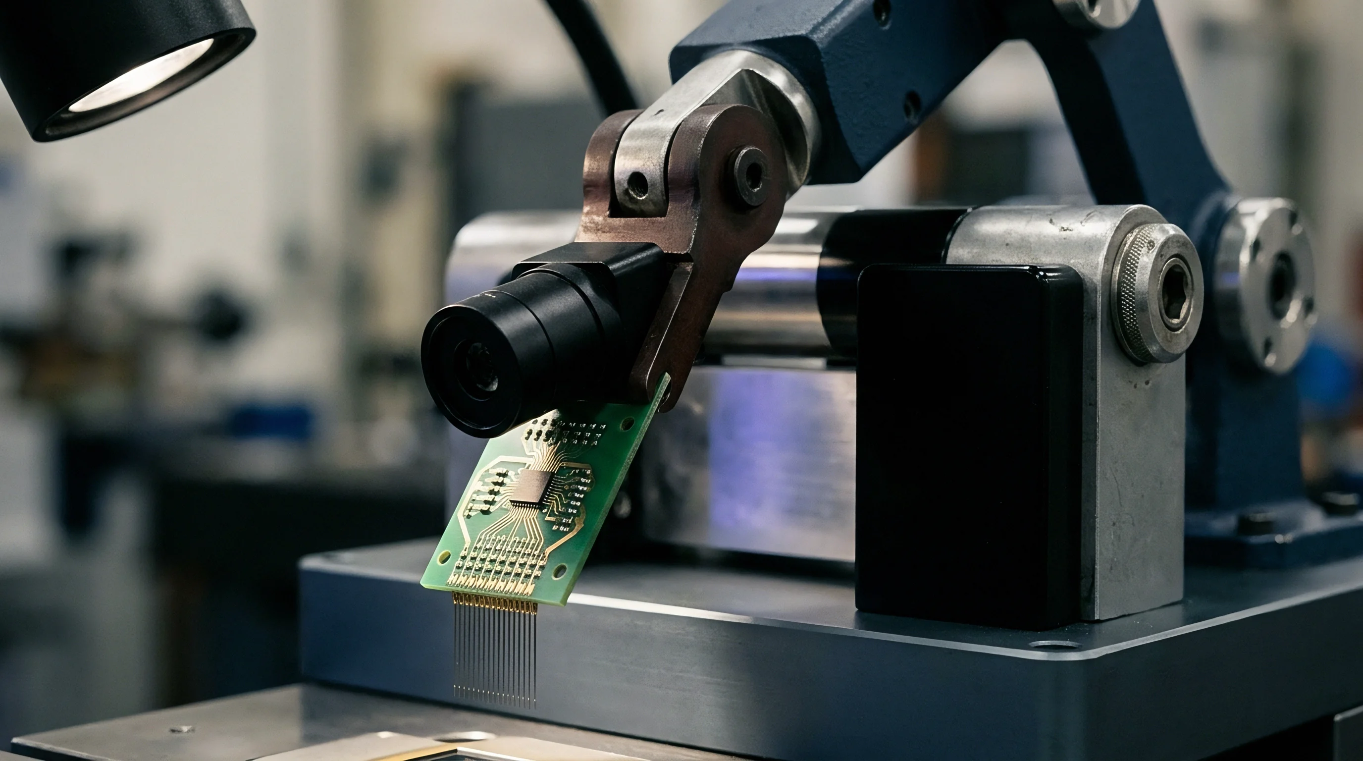
- Photographic evidence photos clear macro imagery highlighting physical housing cracks, terminal pin misalignment, or seal defects.
Commercial Chargebacks and Yield Recovery
Sourcing agreements specify financial deductions when incoming lot yield falls below agreed thresholds. Contracts mandate that suppliers pay sorting labor fees, bench calibration time, and return freight costs for rejected shipments. Establishing intake verification baselines creates explicit legal documentation that shifts quality costs back to component vendors.
Sourcing teams enforce contract clauses that require suppliers to replace rejected lots within ten business days to prevent assembly plant line stoppages. Archiving calibration baseline records inside the central quality management system provides the factual backing required during vendor invoice audits.