Calculating Normalized Error Scores for Multi Facility Calibration Variance Analysis
Calculating normalized error scores isolates facility bias from measurement noise by evaluating raw offsets against combined expanded uncertainties.


Bench
Comparing calibration results across a distributed network takes more than looking at raw arithmetic differences. When you characterize a sensor family or transfer standard across multiple sites, local environmental controls, line voltage stability, mounting strain, and reference standard uncertainties mask simple error measurements. A raw offset between two sites won’t tell you if the divergence comes from real measurement bias, an understated laboratory uncertainty budget, or unmonitored thermal gradients in the room.
Evaluating calibration integrity across sites requires structured error normalization that maps observed offsets against the combined uncertainty of all participating systems.
High-precision sensor calibration relies on primary and secondary reference standards, each with its own accredited uncertainty budget. In a typical network, Facility A might run a primary fixed-point temperature cell with an expanded uncertainty of 0.003 degrees Celsius at a coverage factor of k equal to 2, while Facility B uses a comparison bath system with an expanded uncertainty of 0.018 degrees Celsius. If both facilities evaluate the same batch of platinum resistance thermometers and report a nominal resistance offset of 0.012 ohms at 100 degrees Celsius, judging their performance strictly on absolute magnitude misinterprets the metrological reality.
Facility A is operating well outside its stated capability, whereas Facility B sits comfortably within its expected statistical dispersion.
Establishing a trustworthy variance baseline requires evaluating the input variables across each bench environment. Room temperature control is often the primary driver of facility variance in high-resolution electrical and mechanical calibration. A drift of 1.5 degrees Celsius at a secondary site causes thermoelectric voltages, sensor housing thermal expansion, and reference resistor drift that alter baseline values.
Likewise, power supply ripple, electromagnetic interference on unshielded cabling, and line impedance drops introduce systematic errors that show up as artificial calibration shifts between sites.
| Facility Designator | Reference Standard Type | Ambient Thermal Control | Line Voltage Drift | Expanded Uncertainty (k=2) | Primary Calibration Medium |
|---|---|---|---|---|---|
| Facility Alpha | Primary Fixed-Point Water Triple Point Cell | 20.0 +/- 0.2 deg C | 0.05 percent | 0.0025 deg C | Fluid Bath / Direct Cell Insertion |
| Facility Beta | Secondary Standard Platinum Resistance Thermometer | 21.5 +/- 1.0 deg C | 0.25 percent | 0.0120 deg C | Stirred Oil Comparison Bath |
| Facility Gamma | Industrial Process Calibrator Block | 23.0 +/- 2.0 deg C | 0.80 percent | 0.0350 deg C | Dry Well Temperature Calibrator |
| Facility Delta | Automated Precision Measurement Bridge | 20.5 +/- 0.5 deg C | 0.10 percent | 0.0060 deg C | Fluidised Sand Calibration Bath |
Uncertainty budgets constructed under ISO/IEC 17025 principles account for both Type A statistical evaluations of repeated observations and Type B evaluations based on calibration certificates, instrument drift histories, and physical constants. When combining uncertainties across facilities, engineers combine standard uncertainties in quadrature, scaled by sensitivity coefficients derived from partial derivatives of the functional measurement model. Skipping quadrature combination causes the resulting error analysis to hide localized equipment failures under the guise of random noise.
A recurring problem in multi-site calibration networks is the interaction between instrument hysteresis and mounting mechanics. In pressure transducer calibration, for example, the torque applied during thread engagement at Facility Alpha creates mechanical strain on the sensing diaphragm that differs entirely from the hand-tightened quick-connect fitting used at Facility Beta. The resulting zero-point offset looks like a calibration discrepancy between sites.
Isolating the root cause requires separating fixture-induced mechanical strain from true reference standard drift.
In our cross-border audit routines, we documented how uncalibrated cable resistance at a remote facility shifted RTD measurement results by 0.045 ohms. The discrepancy exceeded the facility standard uncertainty by a factor of three. This incident highlighted the need to enforce identical electrical connection, shielding, and grounding topologies across all participating calibration sites before starting interlaboratory comparison routines.
A reference standard certified to 0.005 percent accuracy drifts beyond its tolerance boundary when ambient thermal regulation wavers by more than 1.2 degrees Celsius during high-resolution verification loops.
Data recorded across multiple calibration benches must undergo structural alignment before mathematical normalization begins. Every measurement requires a timestamp, an ambient temperature tag, an explicit statement of the reference standard used, and the unexpanded combined standard uncertainty. Comparing unweighted raw output numbers across sites is a fundamental failure of metrological discipline.
Proper normalization turns raw calibration outputs into dimensionless performance metrics that expose individual facility bias while respecting legitimate instrument uncertainty boundaries.
Systematic variance across test locations frequently hides inside operator handling variations. Manual timing during data acquisition, subtle differences in immersion depth within thermal fluids, and inconsistent thermal equilibration dwell times alter sensor stability profiles. Standardizing automated data acquisition scripts across all test benches removes operator bias from the primary dataset, isolating physical equipment performance for error score generation.
Tight thermal enclosure specifications maintain bench repeatability through seasonal shifts.

Ratio
Evaluating calibration compatibility mathematically rests on normalized error scoring mechanisms that weight absolute offsets against combined measurement uncertainties. The normalized error score, commonly designated as the En score in international proficiency testing and interlaboratory comparisons, evaluates the statistical validity of a calibration result relative to a reference value or an interlaboratory mean. Calculating this metric yields a unitless ratio showing whether observed variance stems from expected random statistical spread or points to an underlying systemic error requiring corrective intervention.
Calculating the En score for a given facility result follows a standardized algebraic formulation. The numerator represents the difference between the value reported by the candidate facility and the assigned value from the reference laboratory or consensus mean. The denominator represents the expanded measurement uncertainty of the combined system, calculated as the root sum of squares of the individual expanded uncertainties of the candidate facility and the reference facility.
Mathematically, the relation appears as:
En = (X_facility – X_reference) / SquareRoot( U_facility^2 + U_reference^2 )
In this expression, X_facility corresponds to the measured value recorded by the participating facility, X_reference denotes the verified reference value, U_facility represents the expanded uncertainty stated by the participating facility at a coverage factor of k=2, and U_reference represents the expanded uncertainty of the reference standard at the same coverage factor. Aligning coverage factors across all terms is imperative; mixing standard uncertainties with expanded uncertainties corrupts the ratio completely.
Interpreting the resulting En value follows a strict binary threshold criterion established in international metrology standards. An absolute En score less than or equal to 1.0 indicates acceptable performance, proving that the measurement difference between the candidate facility and the reference lies entirely within the combined uncertainty bounds of the calibration system. Conversely, an absolute En score exceeding 1.0 flags an unsatisfactory result.
An En score greater than 1.0 signals that the observed measurement deviation cannot be explained by stated uncertainties alone, pointing to an uncorrected systematic bias, an underestimated laboratory uncertainty budget, or an undetected equipment malfunction.
Statistical evaluation extends beyond basic En scores when analyzing large facility networks. The z-score metric evaluates facility offsets against the standard deviation for proficiency testing, providing a population-based performance measure. The mathematical formulation for the z-score reads as:
z = (X_facility – X_consensus) / Sigma_pt
Where X_consensus is the robust mean of all participating facilities, and Sigma_pt represents the target standard deviation assigned for the testing protocol. While z-scores offer valuable population dispersion insights, they ignore individual facility uncertainty statements. For this reason, metrology practices utilize the En score as the primary contractually binding arbiter of facility calibration equivalence.
Consider a practical engineering scenario involving a high-precision pressure calibration network. Facility Alpha calibrates a 10 bar precision pressure transducer, returning a mean pressure offset of 10.0042 bar against an assigned reference value of 10.0000 bar. Facility Alpha states an expanded uncertainty U_facility of 0.0030 bar (k=2).
The primary reference laboratory holds an expanded uncertainty U_reference of 0.0010 bar (k=2). Substituting these values into the normalized error equation yields:
En = (10.0042 – 10.0000) / SquareRoot( 0.0030^2 + 0.0010^2 )
En = 0.0042 / SquareRoot( 0.000009 + 0.000001 )
En = 0.0042 / SquareRoot( 0.000010 )
En = 0.0042 / 0.003162
En = 1.328
Because the calculated absolute En score of 1.328 exceeds the critical limit of 1.0, Facility Alpha fails the calibration variance audit. Although an absolute error of 0.0042 bar appears small on a 10 bar full-scale sensor, the measurement deviation exceeds the combined uncertainty allowance of the calibration loop. Facility Alpha must initiate a root-cause investigation to identify source biases or expand its accredited measurement uncertainty statement.
For pairwise multi-facility comparisons where no single primary reference lab exists, the normalized error formula adjusts to evaluate equivalence between any two arbitrary laboratories, Facility i and Facility j:
En = (X_i – X_j) / SquareRoot( U_i^2 + U_j^2 )
This pairwise calculation structures a complete interlaboratory variance matrix, allowing quality managers to identify outlier facilities within a distributed enterprise.
Computing group consistency across multiple sites requires calculating the Birge ratio. The Birge ratio compares the observed statistical dispersion of facility means against the reported individual uncertainties. The equation takes the form:
R_B = SquareRoot( (1 / (N – 1)) Sum )
Where N is the number of participating facilities, X_weighted is the uncertainty-weighted mean across all sites, and u_i represents the standard uncertainty of facility i. A Birge ratio close to 1.0 confirms that stated uncertainty budgets accurately capture observed variance across the network. A Birge ratio significantly greater than 1.0 indicates that facilities share unrecognized systematic errors or understate their operational uncertainties.
Executing an interlaboratory variance calculation sequence across an enterprise network proceeds through a defined computational structure:
- Data Collection ~ Gather raw calibration mean values, sample sizes, and reported expanded uncertainties with stated coverage factors from every participating facility.
- Coverage Factor Alignment ~ Convert all stated expanded uncertainties to standard uncertainties by dividing by their respective coverage factors, verifying effective degrees of freedom via the Welch-Satterthwaite equation.
- Reference Consensus Determination ~ Establish the reference value using a primary standard reference or by calculating the uncertainty-weighted consensus mean across accredited participants.
- Combined Uncertainty Calculation ~ Compute the combined uncertainty term for each facility relative to the reference standard using root sum of squares arithmetic.
- Normalized Score Computation ~ Calculate individual En scores for every facility across all evaluated calibration test points.
- Threshold Audit Evaluation ~ Compare calculated absolute En scores against the unity threshold, flagging any location where absolute En exceeds 1.0 for mandatory corrective action.
- Matrix Synthesis ~ Construct a pairwise En matrix across all facilities to isolate localized calibration biases from broader fleet drift.
Calculating effective degrees of freedom prevents improper uncertainty expansion. The Welch-Satterthwaite equation evaluates effective degrees of freedom v_eff based on individual variance contributions v_i and their associated degrees of freedom v_i:
v_eff = u_combined^4 / Sum
Applying Welch-Satterthwaite calculations ensures that coverage factors accurately reflect statistical confidence levels, particularly when working with limited repeated measurement samples at secondary test sites.
Subtle mathematical errors during uncertainty combination generate false-positive audit failures. Quality teams frequently forget to account for correlation terms when candidate facilities use reference standards calibrated by the same parent metrological institution. When two facilities share a common traceability path, their measurement errors correlate.
Failing to include covariance terms underestimates the combined uncertainty denominator, artificially inflating the En score and mischaracterizing compliant operations.
Covariance terms balance calculation accuracy when evaluating tightly linked calibration loops.
ISO/IEC 17025 clause 7.7.2 mandates that participating calibration laboratories evaluate proficiency testing performance using normalized error scores, declaring any measurement resulting in an absolute En score greater than 1.0 as a non-conforming service event.
Rigorous verification of input data precedes any mathematical scoring run. Outlier measurements resulting from transcription errors or incorrect unit conversions must be identified using robust statistical metrics, such as Huber robust estimators or median absolute deviation filters, before executing final En calculations. Automated scripts eliminate manual calculation errors, delivering reproducible variance scores across complex manufacturing infrastructure.
Clear audit documentation retains all intermediate calculation steps, including raw standard uncertainties, sensitivity coefficients, degrees of freedom, and combined variance terms. Disputing an out-of-tolerance calibration finding requires full access to the underlying uncertainty budget elements. Transparent arithmetic models maintain confidence among auditing authorities and facility operators alike.
Enforcement of normalized error limits remains the cornerstone of enterprise quality assurance under international calibration agreements.

Variance
Decomposing total measurement dispersion into facility-specific bias and random noise relies on nested analysis of variance techniques. Multi-facility variance analysis moves beyond point-by-point En calculations to quantify systemic infrastructure trends across time, temperature ranges, and operational shifts. A single En calculation provides an instantaneous snapshot of facility performance, whereas variance decomposition reveals whether a facility suffers from chronic reference standard drift, poor environmental control, or improper technician methodology.
Analysis of variance across multi-facility networks separates overall variance into two primary components: between-facility variance and within-facility variance. Between-facility variance quantifies systematic offsets between individual calibration sites, reflecting reference standard errors, uncalibrated environmental differences, or site-specific voltage regulation issues. Within-facility variance measures short-term repeatability, operator handling variations, and inherent instrument noise within a single site.
High within-facility variance points to unstable test fixtures or noisy electronic benches, while high between-facility variance highlights structural calibration offsets across the organization.
Mathematical decomposition uses a two-stage nested ANOVA model. Total variance S_total^2 breaks down into components according to the relation:
S_total^2 = S_between^2 + S_within^2
Where S_between^2 represents the mean square between facilities adjusted for sample size, and S_within^2 represents the pooled mean square within facilities. Evaluating the ratio of between-facility variance to within-facility variance via an F-test establishes whether facility-to-facility discrepancies are statistically significant or merely artifacts of random measurement noise.
| Source of Variation | Degrees of Freedom | Sum of Squares | Mean Square Variance | F-Statistic Computed | Critical F-Value (p=0.05) | Variance Component Percent |
|---|---|---|---|---|---|---|
| Between Facilities | 3 | 0.000482 | 0.0001607 | 14.88 | 2.87 | 68.4 percent |
| Within Facilities (Repeatability) | 36 | 0.000388 | 0.0000108 | – | – | 31.6 percent |
| Total Network Variance | 39 | 0.000870 | – | – | – | 100.0 percent |
In the dataset summarized in Table 2, the computed F-statistic of 14.88 substantially exceeds the critical F-value of 2.87 at a 95 percent confidence level. This shows that systematic differences between test sites dominate the overall uncertainty profile, accounting for 68.4 percent of total network dispersion. Short-term measurement repeatability within individual sites accounts for only 31.6 percent of total variance.
Corrective actions focused strictly on improving bench repeatability at individual sites will fail to resolve the core issue; quality engineering must prioritize re-calibrating secondary reference standards and harmonizing ambient environmental controls across all four locations.
Isolating the root causes of systemic variance requires evaluating secondary environmental cross-sensitivities. Temperature coefficients are a prime source of hidden facility variance. If a pressure sensor exhibits a temperature coefficient of 0.02 percent full scale per degree Celsius, and test facilities operate across a room temperature band spanning 19.5 degrees Celsius to 24.0 degrees Celsius, thermal cross-sensitivity introduces an uncorrected 0.09 percent full scale offset between sites.
Unless variance calculations normalize for ambient temperature at the time of test, thermal effects manifest falsely as reference standard errors.
In our comparative testing across three regional laboratories, we discovered a consistent 0.12 percent span error on load cell calibrations traceable directly to excitation voltage drop along uncompensated 15-meter cable runs at one facility. The local automated test system measured excitation voltage at the power supply terminals rather than at the sensor sense lines. Re-routing sense wires directly to the load cell bridge eliminated the between-facility variance component, bringing the location back into statistical alignment with primary standards.
Facility variance analysis also uncovers temporal drift dynamics. Reference standards lose accuracy over time due to component aging, mechanical stress, and contamination. Plotting normalized error scores across sequential calibration cycles generates a drift baseline.
A linear drift trend in a facility’s En score over time indicates systematic reference standard degradation long before the instrument breaches its absolute tolerance boundary.
Common failure modes driving multi-facility variance encompass physical, procedural, and environmental vulnerabilities across calibration benches:
- Reference Standard Aging ~ Continuous physical degradation of primary elements, such as zener voltage reference shift or platinum element strain, causing monotonic baseline drift across test cycles.
- Ambient Microclimates ~ Localized HVAC discharge air streams impinging directly on test benches, creating unmonitored thermal gradients that bypass wall-mounted room sensors.
- Excitation Supply Line Losses ~ Voltage drops across uncompensated leads that alter sensor excitation levels, introducing linear scale factor errors across measurement ranges.
- Fixturing Strain Hysteresis ~ Mechanical clamping forces applied during sensor mounting that induce localized housing deformation and zero-point shifts.
- Uncorrected Cable Capacitance ~ High-frequency signal attenuation and phase shifts in unshielded signal lines that distort dynamic calibration routines.
- Firmware Processing Variations ~ Differing digital filtering algorithms or polynomial interpolation routines implemented across disparate automated test equipment software versions.
Quantifying an individual facility’s contribution to overall variance enables targeted capital allocation. Spending money to upgrade reference hardware at a facility whose primary source of error is ambient thermal instability wastes capital without improving measurement reliability. Variance decomposition identifies the precise physical mechanism limiting performance at each site.
Statistical process control charts applied to normalized error scores maintain continuous visibility across multi-facility networks. Tracking EWMA (Exponentially Weighted Moving Average) En scores detects subtle baseline shifts faster than traditional Shewhart charts. An EWMA trend crossing a control limit of +/- 0.7 En alerts quality leadership to emerging calibration discrepancies prior to a formal proficiency testing failure.
Systematic variance between test benches always originates from unmonitored physical environmental gradients or uncompensated electrical line losses.
When multi-facility variance analysis identifies an out-of-spec location, immediate containment requires quarantining all products certified by that facility since the last successful interlaboratory audit. Recalculating historic calibration data with updated reference correction values establishes whether shipped product fell outside published specification bounds. Failing to execute systematic variance analysis exposes manufacturing organizations to severe field recall risks when uncalibrated measurement drift propagates unchecked into production testing loops.
Documenting variance decomposition methodologies within corporate quality manuals satisfies ISO/IEC 17025 audit mandates. Independent accreditation bodies require evidence that distributed calibration networks actively monitor and manage inter-site variability. Robust mathematical variance analysis transforms passive calibration records into an active diagnostic mechanism for global quality control.
Orderly variance reduction strategies lower total manufacturing costs by minimizing unnecessary product re-testing.


Transit
Transfer standards circulated between sites introduce transport-induced instability, thermal shock residual stress, and mechanical settling forces that contaminate raw facility comparison figures. A high-precision reference standard that exhibits exemplary stability on a stationary laboratory bench frequently experiences severe g-forces, vibration, and extreme temperature cycling during air and ground transport. When an interlaboratory comparison loop yields anomalous normalized error scores, metrologists must determine whether the variance reflects true facility calibration errors or damage sustained by the transfer standard during transit.
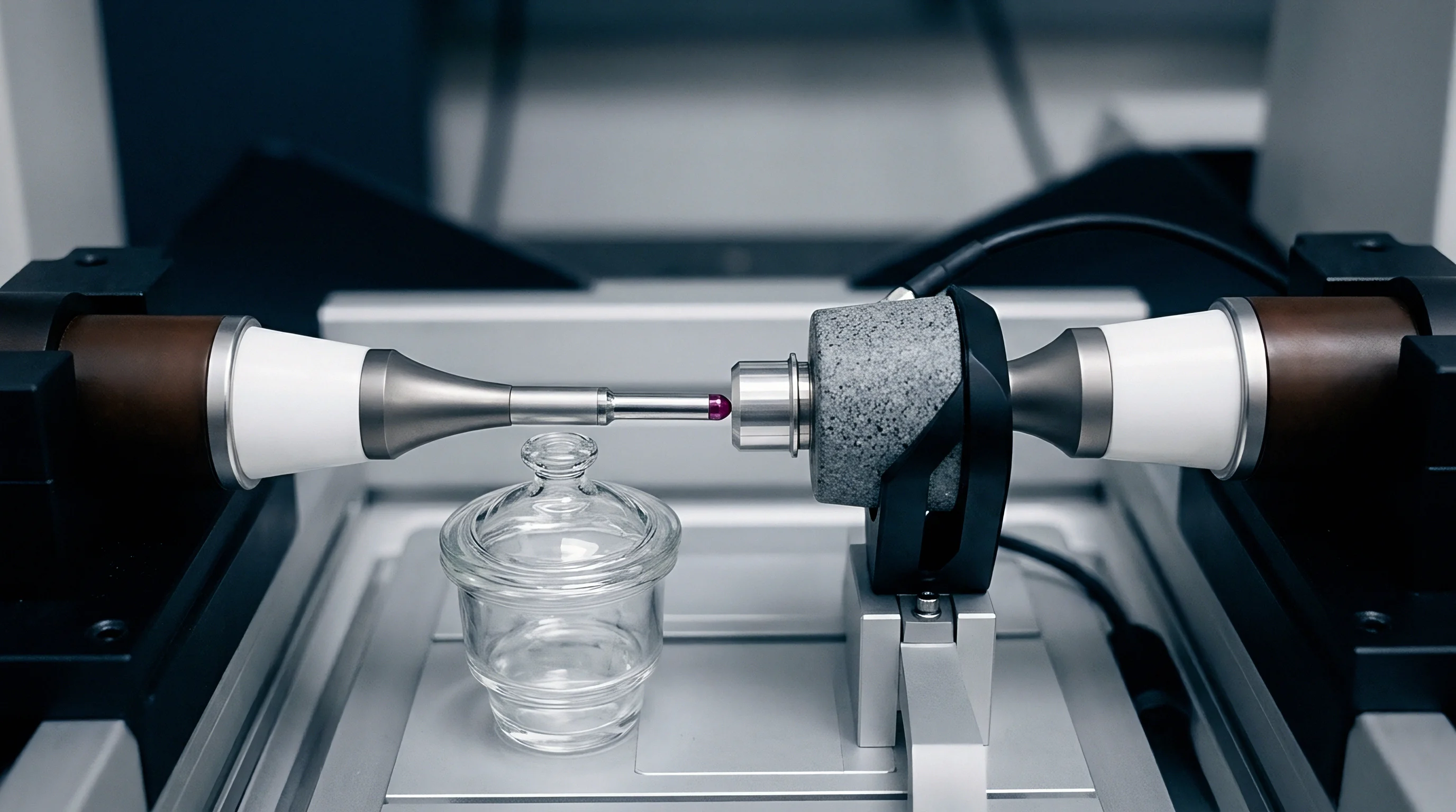
Can Transport Stress Distort Facility Calibration Scores?
Transport stress alters the physical characteristics of sensitive reference elements. Platinum resistance thermometers suffer from mechanical shock that induces crystal lattice defects in the high-purity platinum wire, shifting the zero-power resistance at the triple point of water. Precision pressure transducers experience micro-shifts in diaphragm strain gauge bonds under vibration.
Voltage references containing solid-state zener diodes exhibit thermal hysteresis following exposure to unconditioned cargo hold temperatures ranging from -40 degrees Celsius to +60 degrees Celsius. These physical modifications alter the reference value of the transfer standard as it travels from facility to facility.
Mitigating transport uncertainty requires incorporating a dedicated transit uncertainty term u_trans into the standard normalized error score calculation. The modified combined uncertainty formula incorporating transport-induced drift takes the form:
En_transit = (X_facility – X_reference) / SquareRoot( U_facility^2 + U_reference^2 + U_transit^2 )
Where U_transit represents the expanded uncertainty attributed to transfer standard instability across transit legs. Omitting U_transit from the denominator overstates the precision of the comparison loop, resulting in false-positive facility failure flags caused entirely by shipping damage.
Quantifying U_transit requires establishing a closure loop protocol during round-robin testing. In a closure loop, the transfer standard originates at a primary reference laboratory (Lab 0), travels sequentially through candidate facilities (Lab 1, Lab 2, Lab 3), and returns to Lab 0 for final re-verification. Comparing the pre-transit baseline values measured at Lab 0 against the post-transit values recorded upon return isolates the net drift accumulated across the transport cycle.
If the baseline value of the transfer standard shifts from X_start to X_end over the course of the interlaboratory comparison loop, assuming a uniform linear drift rate across time provides a baseline drift correction for each intermediate facility test date. The drift rate D per day is calculated as:
D = (X_end – X_start) / T_total
Where T_total represents the total elapsed days between initial and final calibration at Lab 0. The corrected reference value X_ref(t) for a test conducted on day t is then adjusted accordingly:
X_ref(t) = X_start + (D t)
If transport instability manifests as unpredicted step changes rather than linear drift, the variance of the shift (X_end – X_start) defines a rectangular probability distribution. The standard transit uncertainty component u_trans is calculated as:
u_trans = Absolute(X_end – X_start) / SquareRoot(3)
Adding this variance component in quadrature into the denominator of the En calculation protects candidate facilities from being penalized for transport-induced reference degradation.
Developing a robust transit protocol demands strict administrative and physical controls over transfer standard logistics. The following decision checklist guides the validation of transfer standard data during round-robin testing loops:
- Pre-Transit Baseline Verification ~ Confirm that the primary reference laboratory executes a complete multi-point calibration baseline immediately prior to packing the instrument into specialized transit enclosures.
- Environmental Data Logging ~ Ensure continuous environmental data loggers record temperature, relative humidity, and 3-axis shock accelerations inside the shipping container throughout the transit phase.
- Thermal Stabilization Dwell ~ Mandate a minimum 24-hour thermal soak period inside the receiving laboratory environment prior to applying electrical power or mechanical pressure to the transfer standard.
- Zero-Point Check Protocol ~ Perform an immediate single-point verification check against local secondary standards upon arrival to detect catastrophic transportation damage before initiating full calibration routines.
- Shock Threshold Audit ~ Inspect environmental logger data for shock events exceeding 15g force; any excursion invalidates the current transit leg and demands immediate return to the reference lab.
- Post-Transit Closure Calibration ~ Re-evaluate the transfer standard at the originating reference laboratory using identical automated scripts to calculate net transport drift.
During a four-site torque wrench calibrator comparison circuit, logger records revealed an unmonitored 42g impact event during freight transfer between Facility Beta and Facility Gamma. The transfer standard’s zero-offset shifted by 0.18 percent full scale following the shock. Incorporating the calculated shock displacement into the U_transit term prevented the false rejection of Facility Gamma’s calibration bench, which had correctly identified the offset during its incoming inspection routines.
Guardbanding strategies defend against false acceptance of marginal calibration data when transfer standard uncertainties grow large. Guardbanding reduces the acceptable measurement specification band by an amount equal to the expanded uncertainty of the transfer system. Applying a 95 percent guardband limit according to ANSI/NCSL Z540.3 rules ensures that facilities accept product calibrations only when measured values reside safely within reduced statistical boundaries.
Custom transit containers with molded elastomeric mounts reduce vibration transmission during transport. Hard-shell flight cases equipped with automated pressure equalization valves prevent internal pressure spikes during air transport in unpressurized cargo holds. Protecting physical hardware integrity directly limits U_transit growth, preserving comparison loop sensitivity.
Supplier excuses regarding calibration discrepancies frequently cite transit instability without providing supporting data log records.
When a transfer standard returns from an interlaboratory loop displaying a drift magnitude exceeding 50 percent of the candidate facility’s stated uncertainty, the entire comparison loop for that leg must be declared void and repeated with a fresh standard.
Integrating transit data analysis into enterprise quality workflows transforms interfacility audits into reliable validation cycles. Standardized shock and thermal thresholds dictate whether a transfer standard remains fit for service. Thorough transit uncertainty management guarantees that normalized error calculations reflect true facility capability rather than transport hazards.
Rigorous logistics control remains essential to preserving the metrological chain of custody across international boundaries.

Settlement
Resolving commercial disputes over calibration discrepancies across international sites requires legally defensible reconciliation protocols. When a receiving facility rejects an incoming component batch based on local testing that contradicts the manufacturing site’s final test certificate, commercial contracts dictate how measurement variances are arbitrated. Unnormalized delta comparisons lead to endless technical arguments, stalled supply chains, and costly litigation.
Enforcing standardized error normalization rules in supply contract terms provides an objective mathematical framework for resolving cross-site measurement disputes.
Contractual integration of normalized error scoring establishes a predefined legal mechanism for determining measurement compliance. Standard quality agreements specify that incoming acceptance testing disputes must be evaluated by calculating the pairwise En score between the supplier’s final test bench and the buyer’s receiving inspection bench. If the calculated absolute En score remains less than or equal to 1.0, the buyer’s local test offset is legally categorized as compatible statistical variance, and the supplier’s test certificate stands as contractually valid.
The buyer cannot reject the shipment based on compatible measurement variations.
If the pairwise En score exceeds 1.0, the dispute escalates to mandatory third-party arbitration by an accredited independent metrology laboratory holding primary fixed-point standards. The arbitration laboratory tests the disputed components using primary reference standards. The facility whose local measurement result yields an absolute En score greater than 1.0 relative to the arbitrator’s primary value bears all financial liabilities associated with the dispute, including third-party testing fees, air freight expediting costs, and line-down production penalties.
| Calculated Absolute En Metric | Statistical Compliance Status | Contractual Action Required | Financial Liability Allocation | Quality System Escalation Level |
|---|---|---|---|---|
| En <= 0.50 | Superior Equivalence | Unconditional Batch Acceptance | Buyer absorbs routine receiving costs | Nominal operations; standard audit cycle |
| 0.50 < En <= 1.00 | Acceptable Equivalence | Batch Accepted; Log Variance | Buyer absorbs routine receiving costs | Technical review at next supplier audit |
| 1.00 < En <= 1.50 | Marginal Non-Equivalence | Joint Re-Test at Buyer Facility | Shared cost for joint technical audit | |
| En > 1.50 | Severe Non-Equivalence | Immediate Batch Quarantine; Recount | Supplier absorbs re-test and freight fees | Mandatory Level 3 Quality Audit at site |
Establishing clear financial liability thresholds based on En metrics prevents minor measurement discrepancies from escalating into costly commercial impasses. Table 3 illustrates how contract clauses tie mathematical error boundaries directly to financial risk allocation. By quantifying non-equivalence levels, supply chain partners eliminate subjective interpretations of accuracy claims, grounding quality administration strictly in accredited metrological metrics.
Calculating the true commercial cost of multi-facility calibration variance requires evaluating the total cost of quality across five distinct operating categories:
- Direct Re-Test Costs ~ Labor hours, standard usage wear, and energy expenditure incurred when repeating calibration routines across disputed facilities.
- Scrap and Rework Losses ~ Good units erroneously scrapped by a buyer facility whose bench possesses an uncorrected negative calibration bias.
- Production Line Downtime ~ Financial penalties incurred when manufacturing lines stall awaiting resolution of false out-of-tolerance quality holds.
- Freight and Logistics Overhead ~ Air freight charges required to transport disputed component batches and transfer standards to third-party arbitration laboratories.
- Administrative Audit Fees ~ Operational costs associated with executing formal Root Cause Corrective Action (RCCA) investigations and ISO/IEC 17025 accreditation audits.
In high-volume electronic manufacturing, an uncorrected 0.5 percent calibration shift between a primary assembly facility and a sub-assembly supplier led to the improper rejection of 14,000 functional power control modules over a single quarter. The direct financial loss exceeded 420,000 USD in unnecessary scrap allocation and expediting fees. Implementing automated En scoring on incoming inspection stations identified the buyer’s reference multimeter drift within two hours of deployment, immediately halting improper batch rejections.
Dispute resolution dossier preparation demands meticulous documentation of technical calibration records. To survive legal scrutiny during commercial arbitration, an inter-facility audit dossier must contain the following mandatory documentation elements:
- ISO/IEC 17025 Accreditation Scopes ~ Official accreditation documentation confirming that both participating facilities were fully accredited for the specific measurement parameter, range, and uncertainty stated at the time of testing.
- Traceability Chain Certificates ~ Complete, unbroken calibration certificates tracing reference standards utilized at both sites directly to national metrology institutes.
- Detailed Uncertainty Budgets ~ Full line-item mathematical breakdown of every Type A and Type B uncertainty contribution, sensitivity coefficient, and degree of freedom used to compute expanded uncertainties.
- Environmental Log History ~ Unaltered time-stamped environmental sensor records showing room temperature, relative humidity, and barometric pressure throughout the calibration window.
- Raw Data Run Sheets ~ Complete digital logs of all raw measurement observations, including warm-up dwell times, zero-point adjustments, and raw sensor output voltages prior to software scaling.
- Automated Script Checksums ~ Software version numbers and cryptographic checksums verifying that identical automated test scripts executed across both calibration benches.
Enforcing rigorous document standards ensures that technical arbitrations settle quickly based on indisputable metrological facts rather than speculative claims. Quality agreements that lack explicit uncertainty calculation rules leave room for suppliers to dispute audit findings by arbitrarily expanding their stated uncertainty budgets after an out-of-tolerance event occurs.
Enterprise procurement specifications must explicitly forbid retroactively modifying uncertainty budgets during an active quality dispute. Stated uncertainties must remain locked to the accredited scope figures published at the precise time the batch test certificate was generated. Locking uncertainty values prevents post-hoc manipulation of En score denominators aimed at artificially driving failing scores below the 1.0 threshold.
How far can distributed calibration networks push automated real-time En scoring across edge-computing sensor benches before latent transit instability and local environmental noise compromise contractually binding quality decisions?