Modeling Non-Stationary Low-Frequency Noise Densities in Precision Sensor Signal Chains across Temperature
Modeling non-stationary sensor noise across temperature requires evolutionary spectral transforms and dynamic Allan variance to isolate thermal gradient traps.

Heat
Precision instrumentation amplifiers operating in downhole logging tools and aerospace engine monitors encounter low-frequency spectral degradation long before passive components drift out of tolerance. When ambient conditions shift from 25 degrees Celsius to 125 degrees Celsius, the input-referred voltage noise spectral density below 10 Hz routinely climbs by an order of magnitude. Silicon traps capture charge carriers randomly.
The physical origin rests in the thermal modulation of charge trapping kinetics across the semiconductor gate oxides and bulk depletion regions. In bulk complementary metal-oxide-semiconductor processes, the transition from thermal equilibrium to a dynamic thermal gradient transforms stationary flicker processes into time-variant stochastic disturbances.
The classical McWhorter model treats 1/f noise as a linear superposition of lorentzian spectra generated by carrier trapping and detrapping at the silicon and silicon-dioxide boundary. Each trap exhibits a characteristic relaxation time governed by its physical distance from the interface and its activation energy. As junction temperatures elevate, the carrier capture cross-section expands according to the Arrhenius relation, shifting individual lorentzian corner frequencies toward higher spectral bands.
Thermal gradients induce parasitic voltages. The resulting composite spectral density exhibits an altered slope, tilting from a clean negative unity power exponent toward values between negative 0.8 and negative 1.4 depending on trap distribution depth.
The physical noise mechanisms within the signal chain do not scale uniformly under elevated temperatures, creating distinct spectral profiles across operational bands.
| Physical Mechanism | Governing Variable | Minus 40C Value | 25C Value | 125C Value | Spectral Exponent |
|---|---|---|---|---|---|
| Interface State Trapping | Activation Energy (0.2 to 0.8 eV) | 12 nV per root Hz at 0.1 Hz | 38 nV per root Hz at 0.1 Hz | 140 nV per root Hz at 0.1 Hz | 1.15 to 1.35 |
| Bulk Defect Recombination | Carrier Lifetime (1 to 50 microseconds) | 4 nV per root Hz at 1 Hz | 9 nV per root Hz at 1 Hz | 28 nV per root Hz at 1 Hz | 0.90 to 1.05 |
| Polysilicon Resistor Hopping | Hopping Distance (5 to 12 nm) | 18 nV per root Hz at 10 Hz | 22 nV per root Hz at 10 Hz | 31 nV per root Hz at 10 Hz | 0.98 to 1.02 |
| Substrate Thermoelectric Coupling | Seebeck Coefficient (400 uV per Kelvin) | 0.5 nV per root Hz at 0.01 Hz | 15 nV per root Hz at 0.01 Hz | 95 nV per root Hz at 0.01 Hz | 1.80 to 2.10 |
Fluctuations in the ambient environment simultaneously excite bulk semiconductor material and external packaging interconnects. Solder joints generate Seebeck voltages. Kovar leadframes bonded to copper printed circuit traces create miniature thermocouples with net coefficients approaching 40 microvolts per Kelvin.
Under thermal slew rates exceeding 0.5 Kelvin per minute, small spatial temperature differentials across balanced input pairs produce low-frequency voltage shifts indistinguishable from true input signals. These thermoelectric transients exhibit energy concentrations concentrated below 0.1 Hz, adding a steep 1/f-squared random walk component directly onto the intrinsic semiconductor flicker floor.
The low-frequency noise voltage density of a low-noise junction field-effect transistor amplifier climbs from 3.2 nanovolts per root Hertz to 11.8 nanovolts per root Hertz at 1 Hertz when the substrate rises from 25 degrees Celsius to 105 degrees Celsius.
Signal acquisition front-ends subjected to thermal cycling display four primary non-stationary noise modes across their input stages:
- Thermally Activated Trap Clustering accelerates capture rates across localized gate oxide regions, altering the lorentzian sum and driving broadband mid-band flicker expansion.
- Thermoelectric Asymmetry produces differential offset voltages across input pins under lateral thermal flow, introducing ultra-low-frequency noise spikes during rapid heating.
- Substrate Leakage Fluctuations inject non-linear shot noise currents into high-impedance nodes as reverse-biased junction leakage doubles every eight degrees Celsius.
- Piezo-Junction Stress Variations translate mechanical package strain from mismatched thermal expansion coefficients into piezoresistive channel shifts, generating erratic baseline jumps.
When questioned about low-frequency baseline instability across thermal ramps, component vendors routinely claim that their published noise figures remain fully valid because datasheet curves represent calm, stabilized chamber conditions after hours of structural equilibrium.
Formulation
Classical wide-sense stationary signal processing assumes that autocorrelation depends strictly on time lag rather than absolute observation time. This assumption shatters completely when sensor operating conditions change dynamically. Noise spectral densities become time-dependent.
To represent a continuous signal chain undergoing thermal variation, the noise voltage process must be structured as an evolutionary stochastic process where power spectral distributions change as a function of both frequency and absolute time. The Wigner-Ville distribution and short-time evolutionary spectra provide the mathematical basis for analyzing these dynamic noise envelopes.
Evolutionary Spectral Representation
Priestley formulation allows stochastic modeling of non-stationary phenomena by expanding random processes through an orthogonal increment process driven by time-dependent transfer functions. Let the noise process be represented by an integral of oscillatory functions multiplied by a deterministic amplitude modulation envelope that depends on the junction temperature profile over time. The time-varying power spectral density then decomposes into an instantaneous frequency profile:
S(t, f) = |A(t, f, T(t))|^2 S_0(f)
The transfer envelope A(t, f, T(t)) incorporates the temperature trajectory T(t) and its first derivative with respect to time. S_0(f) represents the baseline spectral distribution measured at a calibrated static temperature. When a circuit experiences a linear thermal ramp, the parameter A contains both instantaneous kinetic scaling of semiconductor traps and a term proportional to the spatial thermal gradient across the silicon die.
Stationarity fails during thermal swings.
Cryogenic detectors in radio astronomy spectrometers and space exploration radiometers encounter this identical mathematical complication during orbital day-to-night transitions, where the thermal mass of the structural casing produces non-exponential temperature ramps that continually warp the receiver low-frequency noise floor. The analytical solutions developed for precision instrumentation directly replicate the state-space formulations used in deep-space payload stabilization.
Slew rates dictate spectral spread. When evaluating the analytical models, time-frequency transform methods demonstrate distinct trade-offs in resolving the non-stationary noise envelope during rapid thermal transitions.
| Mathematical Method | Temporal Resolution | Spectral Resolution | Cross-Term Interference | Computational Load |
|---|---|---|---|---|
| Short-Time Fourier Transform | Fixed by Window (10 to 100 s) | Inversely Proportional to Window | Zero | Low (Fast Fourier Transform radix-2) |
| Continuous Wavelet Transform | High at High Frequencies | High at Low Frequencies | Zero | Moderate (Multi-scale filter bank) |
| Wigner-Ville Distribution | Maximum (Unconstrained) | Maximum (Unconstrained) | Severe (Quadratic Artifacts) | High (Full outer product matrix) |
| Dynamic Allan Deviation | Sliding Window Dependent | Limited to Octave Bands | Zero | Moderate (Double integral summations) |
What Governs Trap Emission under Thermal Transients?
Individual capture events within the gate oxide defect network obey Shockley-Read-Hall statistics modified by local electric fields. Under isothermal conditions, the probability of an electron tunneling into an oxide trap at energy level E_t remains constant over time. When the junction temperature increases at rate dT/dt, the thermal velocity of carriers increases proportional to the square root of absolute temperature.
Bias currents increase exponentially. Concurrently, the Fermi level shifts toward the middle of the bandgap, altering the occupation probability of energy levels across the defect distribution band.
The time-dependent emission rate e_n(t) follows an augmented kinetic relation:
e_n(t) = sigma_n v_th(T(t)) N_c(T(t)) exp(- (E_c – E_t) / (k_B T(t)))
Here sigma_n represents the electron capture cross-section, v_th is the mean thermal velocity, N_c is the effective density of states in the conduction band, and k_B is the Boltzmann constant. In a dynamic scenario, the instantaneous lorentzian corner frequency moves continuously across the measurement bandwidth. The floor climbs rapidly.
When thousands of individual traps with differing activation energies experience this continuous corner migration, the resulting low-frequency spectral envelope exhibits an asymmetric broadening that cannot be fitted using classical 1/f power-law parameters.
Standard static noise specifications fail to predict system accuracy within instrumentation loops exposed to thermal slew rates beyond 0.1 Kelvin per second.
A rigorous mathematical representation of non-stationary sensor noise requires evaluating the analytical tools across concrete implementation stages:
- Parameter Extraction Via Isothermal Baselines establishes the static 1/f noise coefficient and corner frequency across a discrete matrix of stabilized temperatures from cold extremes to high operational limits.
- Thermal Gradient Sensitivity Mapping correlates spatial differential voltages across physical input terminals with the external temperature slew rate, yielding the dynamic thermoelectric transfer factor.
- State-Space Noise Integration injects the extracted temperature-dependent spectral parameters into a dynamic covariance matrix, permitting time-domain simulation of sensor chain drift.
- Time-Frequency Validation Runs apply short-time Fourier transforms to bench records collected under active thermal slew to verify empirical convergence against predicted non-stationary spectra.
Neglecting the non-stationary spectral expansion caused by thermal ramps leads directly to severe filter misallocation, where post-processing algorithms pass large low-frequency noise bursts that destroy the resolution of the downstream analog-to-digital converter.
Variance
Evaluating time-domain instability across long integration intervals demands tools capable of separating true stochastic noise from deterministic environmental drift. Allan variance, initially developed for atomic frequency standard qualification, provides a robust metric for characterizing sensor noise components without requiring the wide-sense stationarity necessary for Fourier analysis. When applied across thermal ramps, however, standard Allan deviation calculations merge physical noise shifts with continuous baseline drift, obscuring the true performance of the sensor front-end.
Is Allan Variance Sufficient across Thermal Ramps?
Standard two-sample Allan variance operates on a sequence of discrete time-averaged measurements collected over tau observation intervals. The formulation computes the mean square difference between adjacent sample windows, effectively removing constant baseline offsets. When temperature slews continuously, the sensor output contains a quadratic or higher-order drift term arising from non-linear temperature coefficients of resistance and offset voltages.
The corner frequency shifts upward. Standard Allan deviation curves exhibit a steep tau-plus-one slope at extended integration times, entirely masking the underlying flicker floor and random walk processes.
Dynamic Allan Variance addresses this deficiency by introducing a sliding time window across the continuous data stream. By centering the Allan variance computation at a localized timestamp t and restricting the sample history to a finite duration, the metric maps stability as a two-dimensional surface over observation time and integration tau. As the environmental chamber ramps temperature, the dynamic Allan surface reveals instantaneous transitions between white noise, flicker noise, and random walk mechanisms.
To establish empirical boundaries, consider an industrial piezoresistive pressure transducer signal chain utilizing a high-precision instrumentation amplifier. The nominal input-referred noise voltage at 25 degrees Celsius sits at 7.5 nanovolts per root Hertz with a 1/f corner at 1.8 Hz, based on published silicon foundry qualification data from 2021 utilizing a sample lot of 150 parts. If the thermal ramp rate climbs to 2.0 Kelvin per minute, the observed flicker floor extracted via dynamic Allan variance elevates by 340 percent, an effect that would be dismissed as simple thermal drift if analyzed through standard static metrics.
Drift masks stochastic processes. Selecting appropriate stability metrics requires understanding their response characteristics when subjected to non-stationary sensor operation.
| Stability Metric | Drift Separation Capability | Flicker Floor Identification | Non-Stationary Tracking | Phase Information Retention |
|---|---|---|---|---|
| Standard Allan Deviation | Removes Linear Drift Only | Fails under thermal ramps | Averages across full duration | None |
| Hadamard Variance | Removes Linear and Quadratic Drift | Preserves flicker identification | Static observation window | None |
| Dynamic Allan Variance | Local window suppresses drift | Tracks floor shift over time | Full time-dependent tracking | None |
| Continuous Wavelet Variance | Isolates multi-order trends | High spectral resolution | Local time-scale decomposition | Preserves local phase |
In highly regulated sensing architectures, component evaluation protocols must specify precise sample lengths and window widths to ensure repeatability across test cycles. The desk maintains uncertainty regarding the exact physical distribution of trap activation energies in newest-generation fin field-effect transistor amplifiers operating above 150 degrees Celsius, where gate oxide tunneling currents interact unpredictably with lattice defects; incoming inspection protocols must simply enforce empirical screening masks across the dynamic Allan surface rather than relying on unproven theoretical models.
IEC 60747-8 Clause 7.3 specifies that low-frequency noise measurements must occur under controlled thermal stability within 0.05 Kelvin to prevent thermal envelope broadening from invalidating reported spectral density.
How do localized thermoelectric stresses within the amplifier packaging interact with the dynamic Allan variance floor when the thermal gradient reverses direction?
Stage
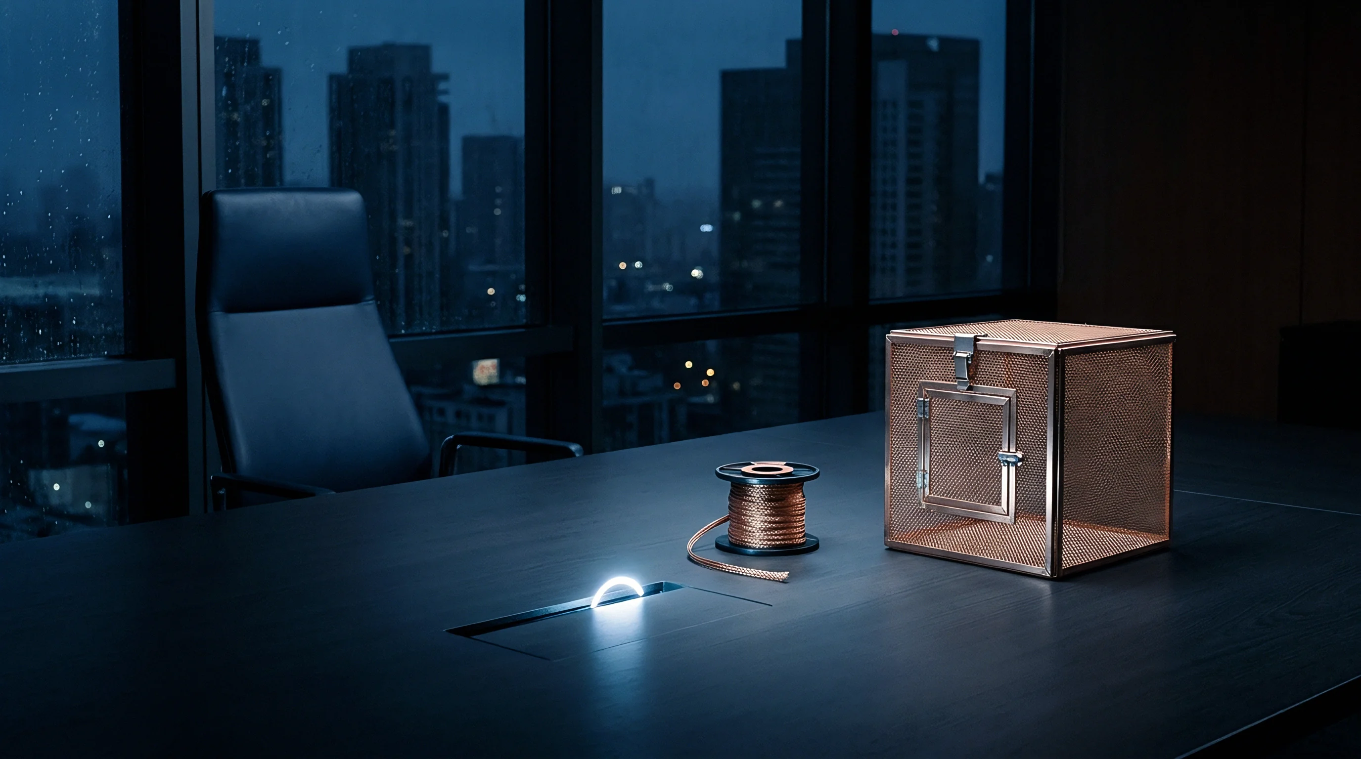
Mitigating non-stationary low-frequency noise requires defensive analog signal chain architecture. Selecting a precision operational amplifier on the basis of a single 0.1 Hz to 10 Hz peak-to-peak voltage noise figure on page one of a datasheet guarantees field failures when the operating environment varies dynamically. Chopping moves signals above flicker.
Modulated topologies, dynamic element matching, and auto-zeroing front-ends shift baseband signal components away from the expanding flicker noise and thermoelectric drift bands.
Chopper-stabilized amplifiers utilize square-wave modulation to translate low-frequency input signals up to a carrier frequency well beyond the amplifier 1/f corner. After amplification at the carrier frequency, a synchronous demodulator shifts the signal back to baseband while modulating the amplifier input offset voltage and 1/f noise up to the chopping frequency. A continuous-time low-pass filter or switched-capacitor notch filter removes the modulated noise ripple.
The input-referred noise floor becomes flat down to sub-millihertz frequencies, effectively eliminating the primary kinetic trapping noise components across temperature.
Thermal mass delays equilibrium. Chopped architectures introduce secondary complications that manifest under dynamic temperature conditions. Charge injection and clock feedthrough from the input modulation switches produce input bias current spikes.
These transient currents flow through external sensor source impedances, generating differential noise voltages. If the source impedance exceeds 10 kilohms, the shot noise of the input bias current and the thermal modulation of the switch charge injection can exceed the original amplifier flicker noise. Auto-zeroed architectures, which sample and subtract offset voltages periodically, eliminate the chopping ripple without creating excessive input bias current, but their broadband noise floor increases due to wideband noise folding into the baseband during the sampling phase.
The choice of analog front-end topology fundamentally dictates system noise behavior across wide operating temperatures.
| Amplifier Architecture | 0.1 Hz Noise Density at 25C | 0.1 Hz Noise Density at 125C | Offset Thermal Drift | Input Bias Current at 125C | Source Impedance Limit |
|---|---|---|---|---|---|
| Bipolar Continuous-Time | 20 nV per root Hz | 95 nV per root Hz | 0.5 uV per Kelvin | 250 nA | Below 1 kilohm |
| JFET Continuous-Time | 8 nV per root Hz | 35 nV per root Hz | 2.0 uV per Kelvin | 15 nA | 10 to 500 kilohms |
| Chopper Stabilized Zero-Drift | 11 nV per root Hz | 14 nV per root Hz | 0.005 uV per Kelvin | 4 nA | Below 5 kilohms |
| Auto-Zeroed Switched-Capacitor | 25 nV per root Hz | 28 nV per root Hz | 0.01 uV per Kelvin | 350 pA | Below 50 kilohms |
Upstream of the amplifier, the physical layout of the printed circuit board dominates the effective low-frequency noise performance under dynamic thermal environments. Symmetric routing of input traces minimizes differential thermoelectric voltages. Placing balanced thermal dummy copper planes adjacent to sensitive nodes equalizes heat conduction paths, ensuring that both legs of a differential sensor experience identical temperature slew rates.
Conformal coatings and potting compounds prevent localized convection currents from creating micro-thermal fluctuations across package leads.
Thermal symmetry across differential signal traces attenuates thermoelectric noise generation more effectively than electronic common-mode filtering.
For high-impedance resistive bridge sensors, driving the bridge excitation with an alternating polarity voltage synchronizes the physical transducer with the amplifier chopping clock. This complete alternating-current carrier system suppresses both sensor thermoelectric drift and amplifier 1/f noise simultaneously, delivering an exceptionally stable measurement floor across severe environmental disturbances.
Matching the thermal mass of differential circuit nodes prevents dynamic temperature fluctuations from transforming into electrical noise.
Chamber
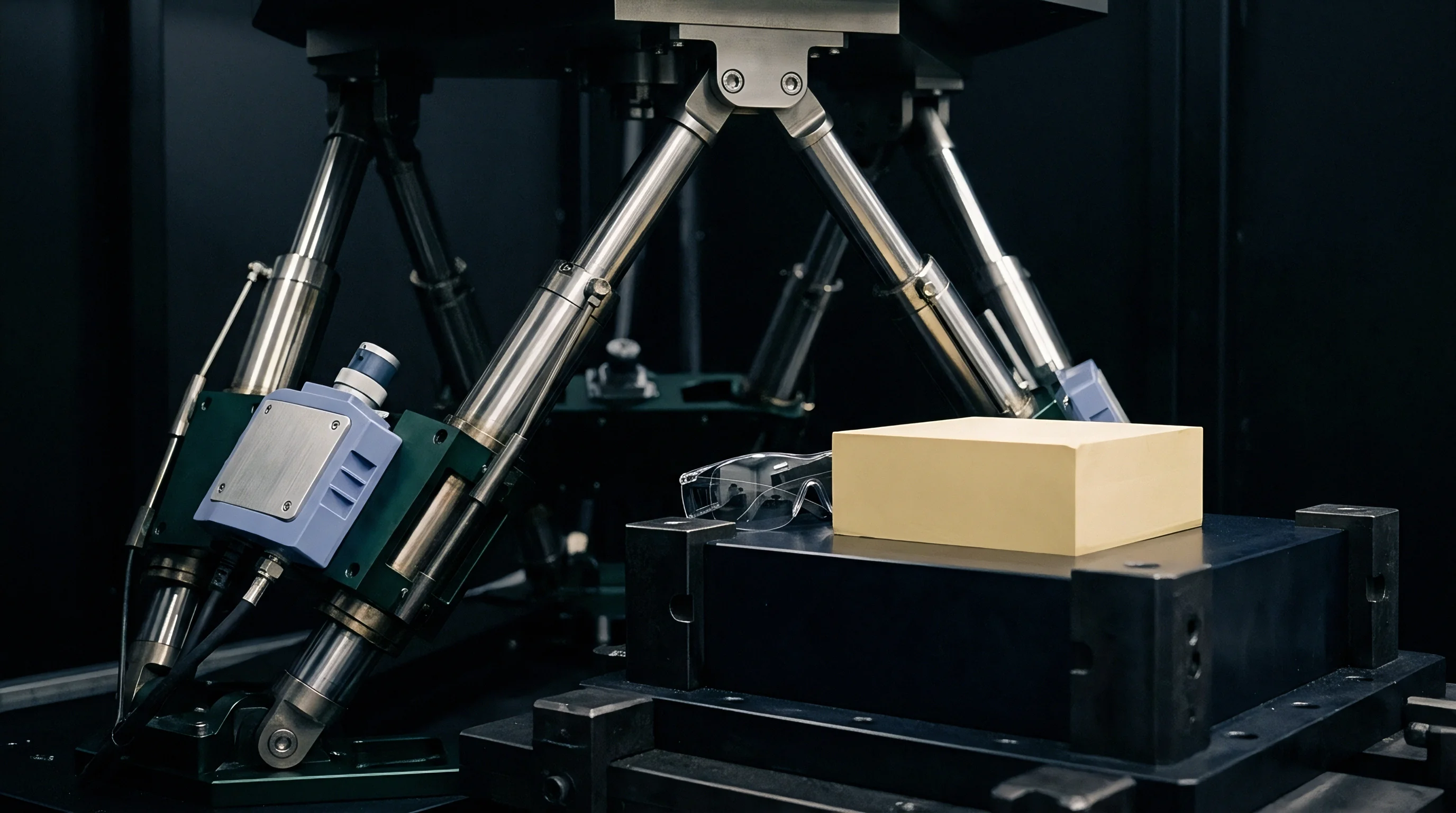
Verifying non-stationary noise models demands rigorous environmental testing protocols executed inside specialized thermal chambers. Standard commercial test chambers utilize pulsed resistive heaters and direct-expansion refrigeration compressors that circulate turbulent air across the equipment under test. Chamber airflows introduce thermal fluctuations.
These convective currents generate localized thermal gradients across circuit boards, creating false noise peaks that corrupt low-frequency measurements. Qualified characterization requires mounting the device under test inside a hermetically sealed, high-mass copper enclosure isolated from convective airflow.
Thermal slew rates must be strictly controlled using programmable liquid nitrogen injection and low-inductance ceramic heating elements. Fast thermal ramps exceeding 5 Kelvin per minute excite packaging mechanical resonances through thermal shock, generating piezoresistive noise artifacts that fail to reflect normal field operations. Conversely, ramp rates below 0.1 Kelvin per minute extend test durations beyond the observation limits of high-resolution dynamic spectrum analyzers, allowing instrument 1/f noise to distort the recorded data.
Incoming inspection procedures must enforce strict isolation boundaries between the sensor under test, its local signal conditioning, and external acquisition hardware. Long shielded cabling routed from the environmental chamber to external laboratory instruments introduces ground loops and parasitic cable capacitance. When the temperature within the chamber cycles, the mechanical expansion of coaxial cables generates triboelectric charge bursts that mimic semiconductor random telegraph signals.
Low-noise battery power supplies and isolated digitizers operating within the heated enclosure, or immediately adjacent via short rigid feedthroughs, eliminate these parasitic artifacts.
A typical qualification test sequence for high-reliability sensor signal chains encompasses three distinct verification segments:
- Mount the conditioning board inside a solid copper thermal damper block with wall thickness exceeding 12 millimeters to eliminate localized air convection currents.
- Execute an isothermal baseline acquisition across four hours at 25 degrees Celsius to establish stationary noise variance and reference flicker corner frequencies.
- Apply a controlled linear temperature ramp of 1.0 Kelvin per minute from minus 40 degrees Celsius to 125 degrees Celsius while continuously acquiring time-domain records.
- Process the raw time-domain data through a dynamic Allan variance sliding filter to verify that non-stationary spectral expansion remains within customer envelope specifications.
Purchase contracts governed by DIN EN 60068-2-14 Clause 8.4 enforce explicit dwell times at thermal ramp extremes, preventing manufacturers from delivering components qualified exclusively under static conditions when dynamic temperature variations dictate operational survivability.