Thermal Zero Drift Correlation for Pressure Sensor Void Fraction Detection
Thermal zero drift distorts two-phase void fraction calculations by creating false differential heads that demand dynamic, high-order polynomial compensation.
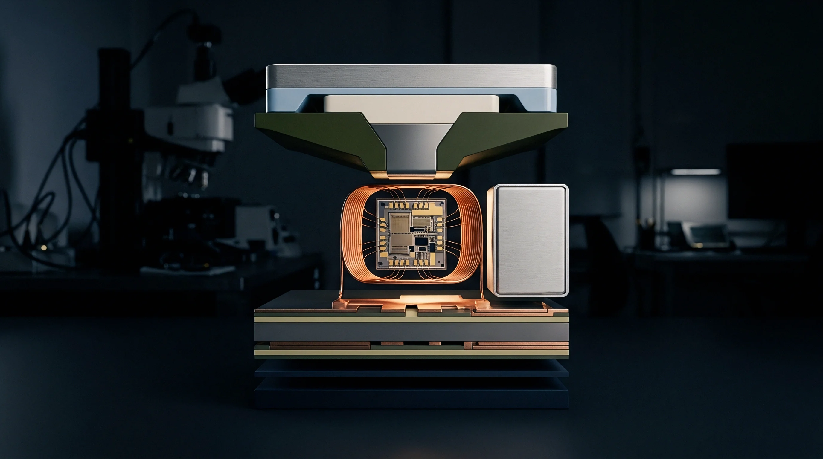
Hydrostatics
Two-phase flow regimes generate differential heads that relate directly to the volumetric distribution of vapor and liquid. In vertical or inclined pipe runs, the measured differential head delta-P across two pressure taps separated by axial distance L reflects the composite mixture density rho-m plus frictional and accelerational losses. When frictional drops remain low relative to liquid mass, mixture density follows a direct linear path from delta-P. Dividing the calculated mixture density by the component single-phase densities yields the cross-sectional void fraction alpha.
Differential pressure transmitters deployed across boiling water channels, flash evaporators, and chemical reboilers monitor this parameter to detect dryout risks or separation efficiencies.
Density governs the differential head. When steam bubbles displace liquid water, gravitational head drops across the elevation span. Transmitters measure this reduction in millimeters of water column or millibars.
In a vertical pipe section with tap separation L of one meter, pure liquid water at two hundred degrees Celsius exerts a hydrostatic drop of approximately eight point four seven kilopascals. Saturated steam at the same temperature exerts roughly zero point one kilopascal over that meter. The difference between those two pressure bounds defines the entire active measurement window for void fraction evaluation.
Any parasitic signal drift shifts the apparent void fraction along that nine-kilopascal span.
A zero shift of forty pascals across a one-meter vertical liquid span induces an undetected void fraction error of zero point four eight percent at two hundred degrees Celsius.
Transmitter stability determines whether the calculated vapor share matches reality or drifts into operational misreadings. Piezo-resistive and capacitance-based differential pressure cells carry internal temperature sensors intended to counteract thermal expansion and resistance drift. Sensor bodies mounted near hot process piping absorb heat via conduction through metal impulse legs and radiant flux from uninsulated flanges.
When process temperatures swing during plant startup, power ramp, or batch cycling, sensor fill fluids expand and internal silicon strain gauges alter their piezoresistive gauge factors.
Void Calculation Mechanics
Spatial averaging across a differential pressure span assumes that acceleration drops and wall friction terms are either negligible or computable via separate hydraulic relations. In upward vertical flow, total differential pressure delta-P equals the sum of the frictional pressure gradient, the spatial acceleration gradient, and the gravitational head rho-m multiplied by gravitational acceleration g and span length L. At moderate liquid velocities below one meter per second, gravity contributes more than ninety percent of the gross differential signal. Void fraction alpha derives from equating mixture density rho-m to the liquid density rho-l multiplied by one minus alpha, plus vapor density rho-v multiplied by alpha.
High void fraction regimes compress the available hydrostatic differential signal into the bottom twenty percent of the sensor span. If an uncorrected thermal zero shift drifts upward by eighty pascals while boiling increases, the acquisition system registers artificially high mixture density. The controller concludes that liquid inventory remains abundant when the conduit has transitioned to annular dryout.
In reboiler loops, this masking leads operators to overdrive heat exchangers, creating localized tube burnouts.
Differential Pressure Sensitivities
Transmitter line pressures alter baseline span characteristics, while thermal shifts attack the zero datum. Piezoresistive diaphragm dies respond to thermal gradients with asymmetric mechanical stress. Even when the sensor body reaches thermal equilibrium, silicon diaphragm membranes exhibit thermal zero coefficients that require cancellation coefficients within the transmitter digital electronics.
The measurement infrastructure tracks rapid void swings only if zero wander stays clamped within narrow bounds. Table 1 catalogs the propagation of zero drift errors across differential pressure spans in saturated water-steam systems at five operating pressures.
| Saturation Pressure (MPa) | Liquid Density (kg/m³) | Vapor Density (kg/m³) | Full Scale Span (kPa) | Zero Drift (Pa) | Resulting Void Error (Absolute %) |
|---|---|---|---|---|---|
| 0.101 | 958.4 | 0.597 | 9.39 | 25 | 0.27 |
| 1.000 | 887.2 | 5.147 | 8.65 | 50 | 0.58 |
| 4.000 | 779.8 | 20.02 | 7.45 | 50 | 0.67 |
| 10.00 | 688.2 | 55.45 | 6.21 | 100 | 1.61 |
| 15.00 | 594.4 | 101.9 | 4.83 | 100 | 2.07 |
Operating plants running at fifteen megapascals forfeit measurement integrity when zero drift climbs past one hundred pascals. At that pressure, the density contrast between liquid and vapor diminishes to less than five hundred kilograms per cubic meter. A small offset error consumes a larger fraction of the available range.
Process safety margins erode when thermal drift goes uncompensated, triggering automatic shutdowns or masking genuine boiling crises.

Diaphragm
Isolating diaphragms transfer process pressure to inner sensing elements via incompressible fill fluids. Metallic diaphragms rolled from Hastelloy C-276, 316L stainless steel, or Monel flex under differential pressure, displacing volume into miniature capillary passages behind the corrugations. Thermal expansion of the fill fluid pushes outward against both process membranes.
If both process diaphragms possessed identical volumetric compliance, identical spring rates, and balanced fill volumes, volumetric expansion would raise internal sensor cavity pressure symmetrically on high and low sides without creating a differential signal.
Silicon oil expands nonlinearly. Manufacturing tolerances prevent perfect symmetry between internal sensor chambers. The high-pressure side chamber routinely holds between two and eight percent more fluid volume than the low-pressure side due to internal geometry variations, sensor die placement, and weld shrinkage.
When ambient or process radiant heat elevates the transmitter housing temperature from twenty degrees Celsius to eighty degrees Celsius, the unequal fluid masses expand by unequal amounts. The stiffer diaphragm resists displacement, forcing a net differential pressure across the silicon sensing die that has no connection to process hydraulics.
How Do Transducer Fills Distort Static Readings?
Filling fluids govern sensor thermal response. Standard differential pressure cells use polydimethylsiloxane oils, fluorocarbon liquids such as CTFE for oxygen service, or synthetic hydrocarbon oils for ultra-high temperature exposure. Each fluid carries an isobaric thermal expansion coefficient between zero point zero zero zero seven and zero point zero zero one two per Kelvin.
The volumetric change delta-V equals the initial volume multiplied by that coefficient and the temperature excursion delta-T.
Internal fluid displacement forces the metallic corrugations to deflect outward against atmospheric or line pressure. Diaphragm stiffness, characterized by the spring rate k-d in newtons per millimeter, translates that deflection into a back-pressure. Because the spring rate of convoluted diaphragms changes as a function of travel and metallurgical work-hardening, the resulting back-pressure delta-P-zero deviates from linear temperature tracking.
Piezoresistive bridges read this pressure as a genuine process imbalance.
Sensor manufacturers mitigate this error by selecting specific diaphragm geometries and filling chemistries. The physical behavior of common fills establishes the baseline drift magnitude:
- High-temperature phenyl-methyl silicone yields predictable volumetric expansion across operating spans between minus twenty and two hundred degrees Celsius, showing minimal polymerization under protracted thermal exposure.
- Chlorotrifluoroethylene fluid presents high density and inert behavior in oxidizing streams, generating higher mass-induced gravitational errors in impulse legs when ambient temperatures fluctuate.
- Proprietary eutectic liquid metals eliminate organic fluid degradation in ultra-high temperature applications, though surface tension shifts introduce micro-hysteresis across low differential pressure spans.
Standard commercial transmitters cite zero temperature coefficients under steady thermal soaking while omitting transient gradient errors between isolation seals.
Asymmetric Impulse Temperatures
Impulse lines connecting pipe taps to the transmitter body introduce additional thermal zero shifts. If the process fluid is hot, sensible heat conducts down the metal piping toward the manifold. In a vertical pipeline, the upper tap often sits within a warm air convection plume while the lower tap remains exposed to cooler ambient cross-drafts.
The fluid column in the high-pressure impulse line can sit at seventy degrees Celsius while the low-pressure line rests at thirty degrees Celsius.
Zero shifts mimic voidage. The density differential between the two impulse fluid columns creates an artificial hydraulic head. In a typical impulse installation with vertical drops of zero point eight meters filled with distilled water, a forty-degree temperature difference between legs generates an error pressure of nearly one hundred and fifty pascals.
The transmitter sensing element reads this difference as lower vessel mass. While field piping insulation and heat tracing reduce these temperature differences, transmitter compensation adjustments are still needed to preserve full measurement stability.

Polynomial
Static zero correction across operating ranges uses mathematical compensation equations embedded in sensor ASIC microcode or flow computer software. The core parameter is the thermal zero drift correlation, which relates observed baseline offset delta-P-zero to temperature measurements gathered at the sensor die and along impulse legs. Simple linear scaling fails to capture the true profile.
Silicon strain gages, mechanical housings, and silicone fill fluids combine to create nonlinear response curves that require polynomial characterization.
A third-order polynomial model maps sensor offset drift caused by membrane thermal gradients across temperature excursions. Equation 1 expresses this baseline correlation:
delta-P-drift(T) = a0 + a1 (T – T-ref) + a2 (T – T-ref)^2 + a3 (T – T-ref)^3
In this formulation, T-ref represents the baseline calibration temperature, typically twenty degrees Celsius, while coefficients a0 through a3 represent empirical calibration parameters determined through thermal chamber cycling. The linear coefficient a1 captures base resistor temperature coefficients. The quadratic term a2 compensates for unequal fill expansion and nonlinear diaphragm deflection.
The cubic coefficient a3 accounts for high-temperature stiffness degradation in diaphragm convolutions.
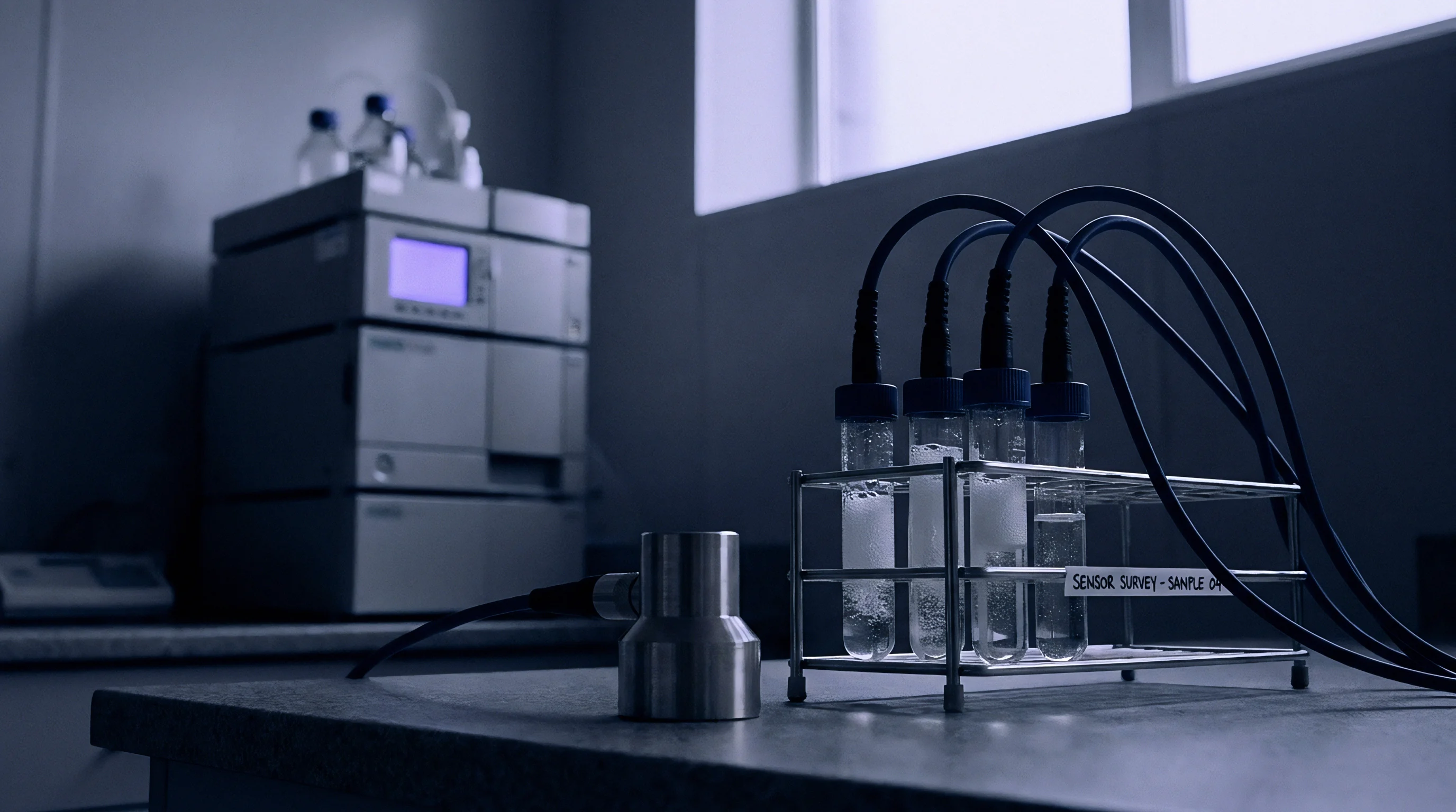
Mathematical Drift Formulation
Static calibration coefficients prove insufficient when transmitter housings experience rapid ambient temperature changes or steep process heat transients. Under dynamic conditions, sensor body temperatures diverge from internal fill fluid temperatures. The on-chip temperature sensor located on the silicon die registers a different thermal state than the fluid chamber or outer Hastelloy diaphragm.
Dynamic compensation adds a rate-of-change term dT/dt to the formulation:
delta-P-dynamic(T, t) = delta-P-drift(T) + tau-th b1 (dT / dt)
Here tau-th represents the thermal time constant of the sensor assembly, typically ranging from twenty-five to one hundred and eighty seconds, and b1 is an empirical heat flux transfer parameter. Ignoring the rate term induces transient drift loops during ambient shifts, causing void fraction spikes that resolve only after the transmitter reaches thermal equilibrium.
Dynamic Lag and Thermal Infiltration
Hysteresis resists simple polynomial fits. Heating a differential pressure cell from twenty degrees to eighty degrees Celsius and returning it to twenty degrees traces a hysteresis loop in zero output. Silicon strain gages exhibit minimal crystal hysteresis, but the Hastelloy diaphragm, silicone oil dissolved gas phases, and elastomeric housing seals retain deformation memory.
Table 2 details typical polynomial compensation residuals across standard temperature intervals for a one-hundred-millibar full-scale differential cell.
| Calibration Model | Polynomial Order | Peak Sensor Drift (Pa) | Maximum Residual Error (Pa) | Peak Void Fraction Uncertainty (%) |
|---|---|---|---|---|
| Uncompensated | None | 340 | 340 | 4.56 |
| Linear Fit | 1st Order | 340 | 68 | 0.91 |
| Standard Quadratic | 2nd Order | 340 | 22 | 0.30 |
| Cubic Hermite Spline | 3rd Order | 340 | 7 | 0.09 |
| Dynamic Rate Corrected | 3rd Order + dT/dt | 340 | 3 | 0.04 |
If the sensor ASIC firmware relies solely on a second-order polynomial without rate correction, transient thermal shocks produce up to twenty-two pascals of unaccounted zero error. In a low-pressure two-phase channel, twenty-two pascals represents a significant distortion of true phase distribution. How field calibration scripts should balance the computational load of high-order multi-point splines against real-time sampling rates remains unresolved across competing instrument architectures.
Rig
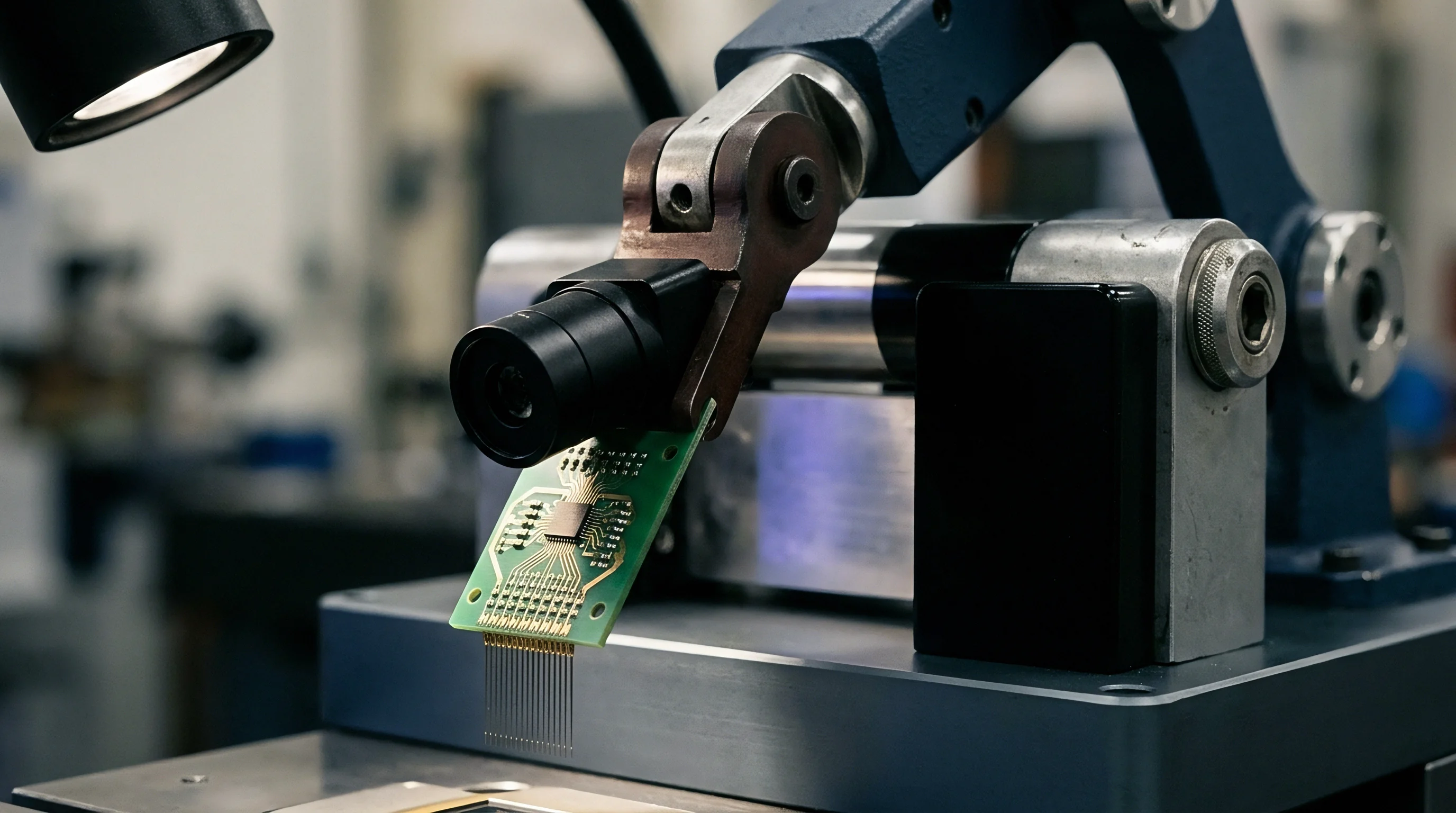
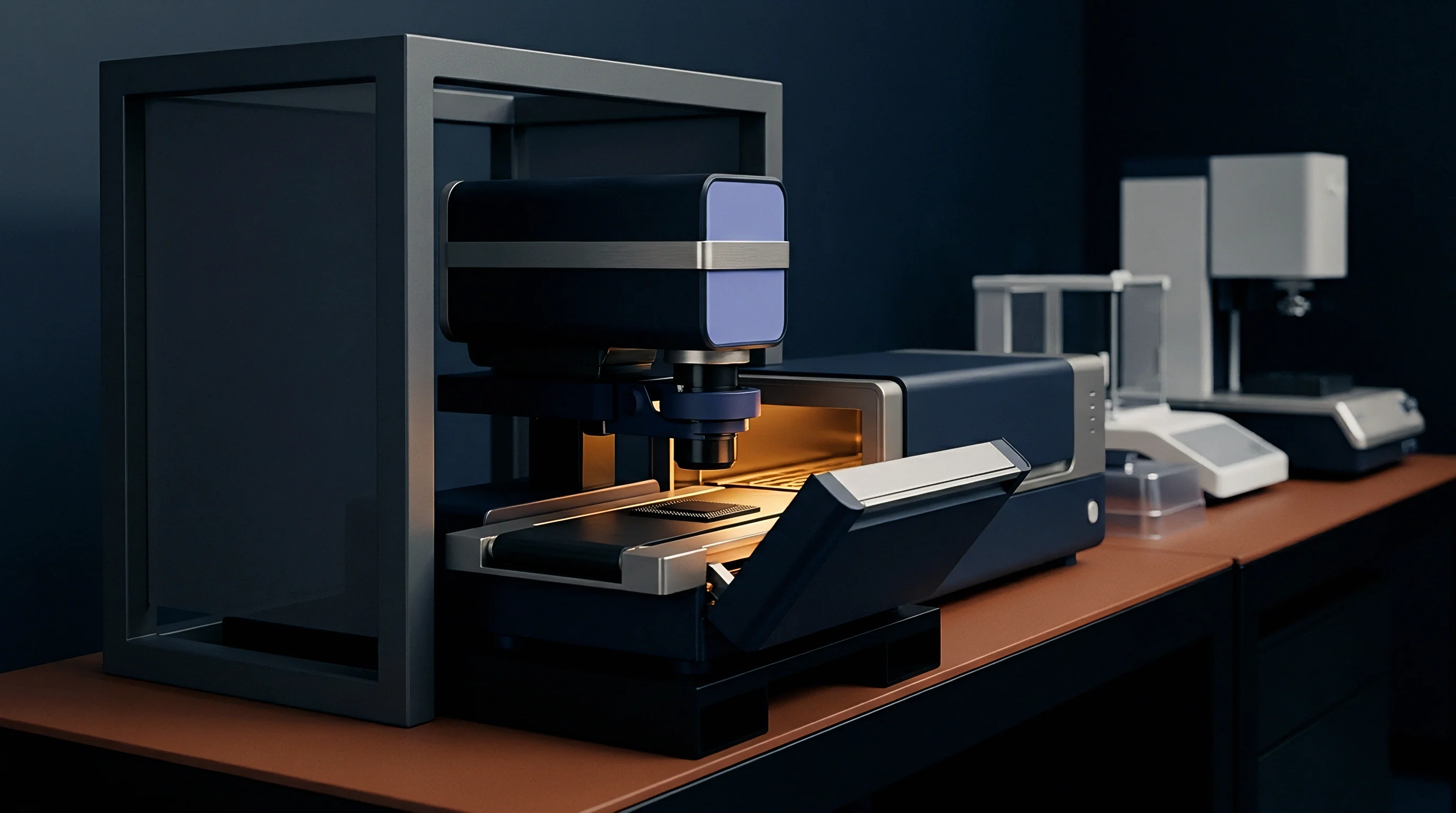
Traceable determination of thermal zero coefficients demands dedicated calibration benches capable of isolating thermal effects from static line pressure and hydraulic turbulence. A laboratory test bench isolates thermal zero drift by subjecting the differential pressure transmitter to controlled temperature profiles while maintaining zero true differential pressure across the high and low process ports. High-accuracy deadweight testers and resonant quartz transfer standards, calibrated under ISO/IEC 17025 accredited procedures, monitor line pressure stability.
Environmental chambers encapsulate the transmitter body and process flanges, controlling air temperatures within zero point zero five degrees Celsius.
Static calibration misses transient shifts. Testing transmitters under uniform chamber heating masks errors that emerge in industrial plants where process fluids are hot and surrounding ambient air is cold. A balanced validation test uses dual oil circulation loops connected to the transmitter process isolating flanges.
One loop circulates thermal oil at process temperature while the transmitter housing remains exposed to circulating ambient air in the chamber. This configuration reproduces real-world thermal gradients across diaphragm necks and capillary seals.

Are Factory Calibration Runs Reproducing Flow Gradients?
Standard manufacturing routines calibrate transmitters inside isothermal air ovens with open ports or equalized manifolds. This process maps uniform sensor die drift but misses temperature gradients along sensor bodies. During true operation, heat conducts through process isolators into one side of the transmitter cell while the opposite side radiates heat to ambient air.
The resulting thermal tilt warps the mechanical housing, producing asymmetrical internal forces that standard isothermal calibration cycles cannot register.
Calibration facilities must execute structured sequences to map these multi-dimensional error spaces:
- The operator mounts the transmitter within the dual-bath rig and stabilizes line pressure at process nominal using nitrogen deadweight standards.
- Both process ports are hydraulically cross-connected through an equalization bypass valve to ensure zero differential input.
- The environmental chamber ramps from twenty to eighty degrees Celsius at a controlled rate of zero point five degrees per minute while continuous data acquisition records sensor offset, die temperature, and case temperature.
- Fluid loop controllers step the high-side process flange to one hundred and fifty degrees Celsius while holding the low-side flange at ninety degrees Celsius, reproducing asymmetric boiling channel tap conditions.
- The operator logs output deviations across three complete thermal cycles to capture mechanical hysteresis and envelope limits.
ISO/IEC 17025 accreditation scopes covering thermal zero coefficients require reporting expanded uncertainty budgets that include environmental chamber thermal stability and deadweight line-pressure regulation.
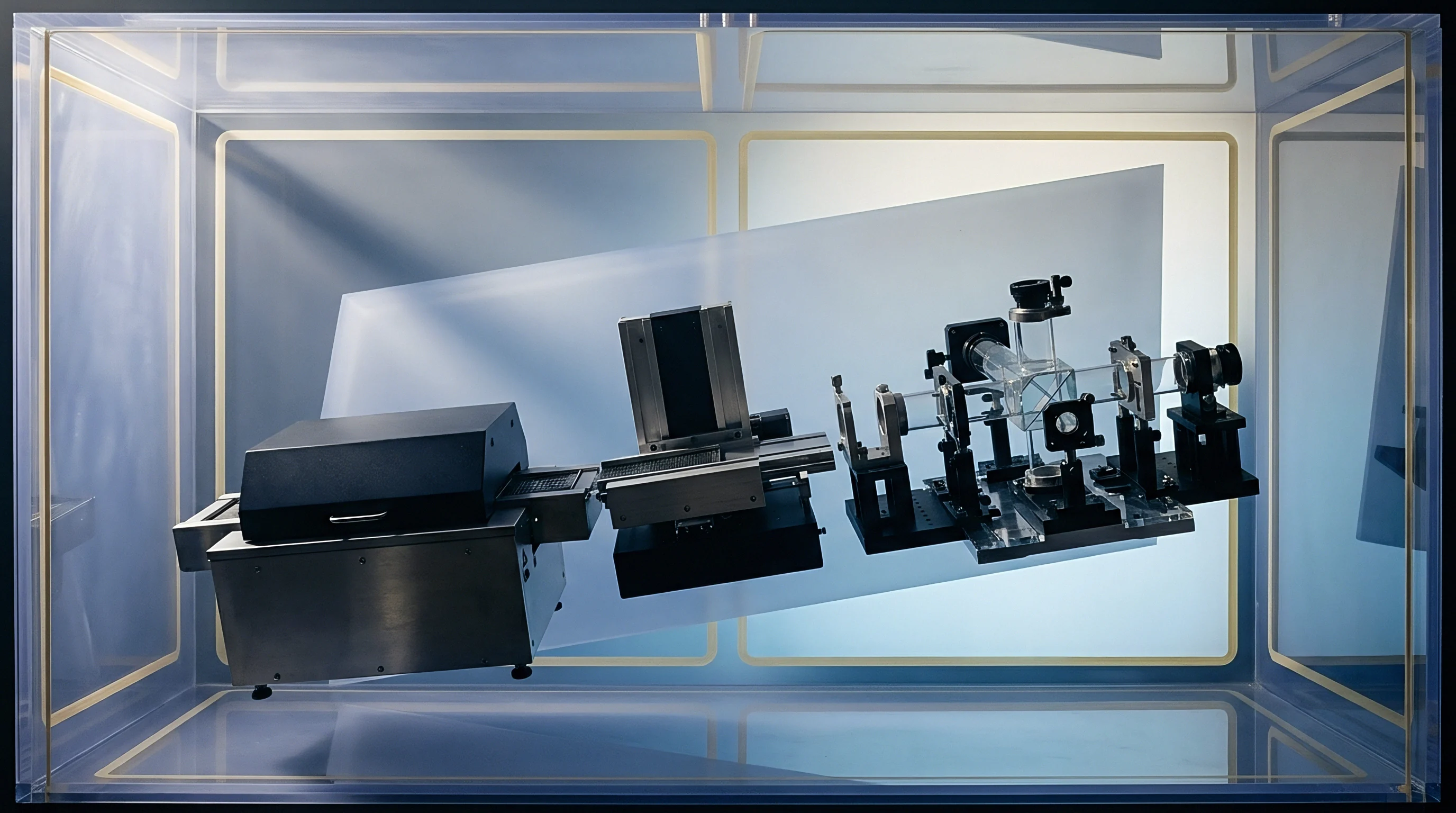
Laboratory Chamber Test Profiles
The sequence of thermal soaking establishes the repeatability of zero parameters. Rapid temperature changes induce thermal shock profiles that expose weaknesses in silicon-to-header glass frit bonding. The test profile holds transmitters at each temperature plateau for at least two hours to confirm that internal fill fluids and mechanical housings have reached thermal equilibrium before offset values are logged.
If readings drift during the final thirty minutes of a soak period, internal stress relaxation remains incomplete.
Over long service intervals, thermal cycling loosens mechanical torque on sensor flange bolts and accelerates fill fluid degassing. Laboratory verification protocols establish the rate at which factory polynomial coefficients drift out of alignment. Section 6.4.3 of IEC 61298-3 specifies that environmental influence testing must quantify zero shift after thermal cycling, and omitting this test clause removes contractual accountability for drift exceeding datasheet envelopes.

Procurement
Specifying differential pressure transmitters for void fraction determination requires direct contractual limits on thermal zero coefficients. Generic process datasheets routinely quote total accuracy figures of plus or minus zero point zero four percent of calibrated span. Those claims apply under factory reference conditions of twenty degrees Celsius and one atmosphere of static line pressure.
The operational thermal zero drift specification often hides in footnote text as an additional error of zero point零 five percent of maximum upper range limit per twenty-eight degrees Celsius shift.
Buying precision requires balancing base transmitter cost against field verification expenses. When differential spans are compressed to ten kilopascals to measure light vapor-liquid mixtures, an unverified zero coefficient will consume the entire project tolerance budget within a minor ambient seasonal shift. Specifying enhanced thermal calibration curves and factory characterization reports adds between twenty and forty-five percent to unit procurement expenses.
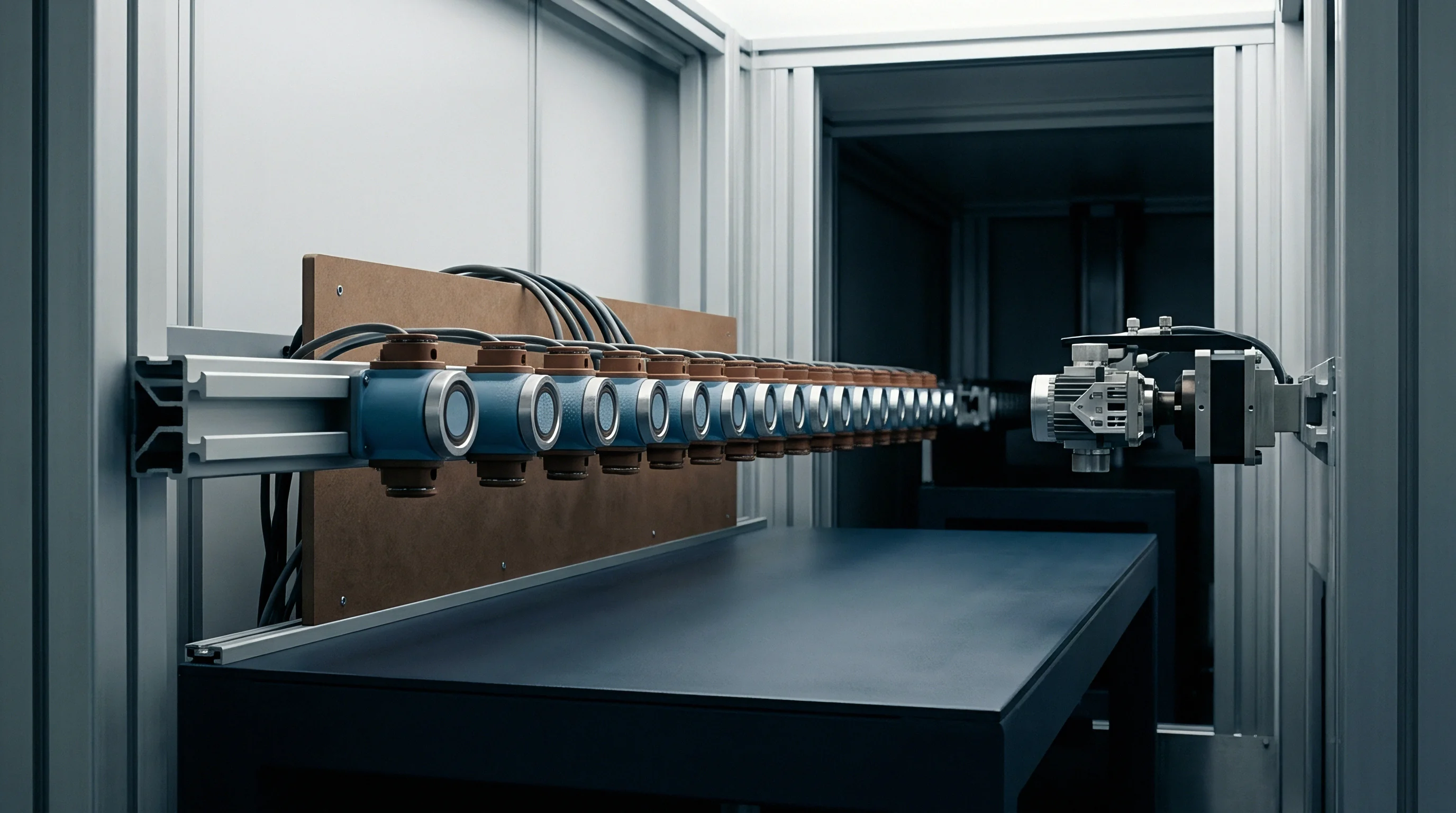
Specification Bands for Process Bids
Engineering bids must distinguish between general process transmitters and units tailored for void fraction detection. Request for Quotation documents must define the maximum permissible thermal zero shift over the complete operating temperature range, rather than accepting ambient-only ratings. Table 3 presents a comparative evaluation of four transmitter specifications, outlining procurement premiums and associated void fraction measurement uncertainties.
| Transmitter Classification | Thermal Zero Specification (% URL / 28 °C) | Zero Drift across 50 °C Swing (Pa) | Uncertainty in Void Fraction (%) | Typical Unit Cost Multiplier |
|---|---|---|---|---|
| Standard Industrial Gauge | ±0.065 | ±116 | ±1.37 | 1.00 |
| Premium Process Grade | ±0.035 | ±62 | ±0.73 | 1.35 |
| Characterized Thermal Trim | ±0.015 | ±27 | ±0.32 | 1.80 |
| Custom Multi-Bath Mapped | ±0.005 | ±9 | ±0.11 | 2.45 |
Process upsets shift line conditions faster than sensor bodies can adapt. When bidding projects that use differential pressure for safety-critical boiling detection, specifying standard industrial grade instruments guarantees frequent false trips or unmonitored boiling crises. The higher capital expenditure for characterized thermal trim grades pays for itself by eliminating routine field rezeroing visits and avoiding unnecessary thermal shutdowns.
Field Rezeroing Protocols and Expense
Maintenance schedules must account for zero wander. Even multi-bath mapped transmitters experience long-term zero aging, typically shifting between ten and thirty pascals per operational year due to fill fluid hydrogen permeation and sensor diaphragm work-hardening. Routine field rezeroing requires technicians to establish an equalized manifold state while the process remains at normal operating temperature.
If maintenance teams rezero transmitters cold during plant outages, the entire thermal zero shift is baked into the operating baseline once the line warms up.
Instrument engineers should require manifold equalizing procedures to take place only after process units attain thermal equilibrium at base operating loads. Selecting transmitters with external non-intrusive zero adjustments and high-stability capillary seals minimizes labor overhead while maintaining void fraction accuracy across seasonal ambient swings. Instruments installed without temperature-compensated zero baselines will drift until the measured void fractions no longer match actual line hydraulics.