Resolving Non-Gaussian Parametric Drift Allocation Disputes across Multi-Tier Sourced Microelectronic Supply Chains
Non-Gaussian drift allocation disputes are resolved by decomposing parametric shifts using empirical quantile bounds and baseline differential tier testing.


Silicon
Microelectronic supply chains assign component fabrication, packaging, and final module integration across geographically dispersed operating entities. When a precision analog integrated circuit or sensor assembly exhibits parametric drift over its operating lifespan, determining which manufacturing tier caused the specification breach presents complex technical challenges. Parametric drift across multi-tier sourcing structures rarely follows standard Gaussian normal distribution curves.
Piezoresistive stress induced by epoxy mold compounds, charge trapping in sub-micron transistor gate dielectrics, interfacial oxidation, and copper wire bond creep introduce asymmetrical skewness and extreme tail populations. Standard root-sum-square tolerance stack-ups assume statistical independence and symmetrical normal distributions. Applying Gaussian assumptions to multi-tier microelectronic drift allocations masks systemic failures, resulting in unresolated commercial disputes between system integrators, outsourced semiconductor assembly and test facilities, and semiconductor foundries.
Packaging stress dominates initial drift.
Assigning financial and technical responsibility across sourcing tiers demands isolating the distinct physical degradation mechanisms that operate at each phase of manufacturing. A precision voltage reference or high-resolution analog-to-digital converter experiences additive parametric shifts throughout its supply chain life. Wafer fabrication introduces baseline lattice defects and gate oxide trap states.
Assembly and packaging impose intense thermo-mechanical stress profiles through differential thermal expansion between the silicon die, leadframe, and encapsulation resin. Surface-mount assembly at the system integrator tier adds thermal shock during solder reflow, altering internal stress state balances. When field failures emerge after thousands of operating hours, separating the underlying foundry drift from packaging strain relief and board-level assembly degradation requires systematic mapping of physical drift vectors to specific empirical probability density functions.

Physical Drivers of Packaging Strain
Direct mechanical forces transferred from epoxy mold compounds into precision die active areas alter carrier mobility through piezoresistive effects. Plastic Quad Flat No-Lead and Ball Grid Array packages undergo volumetric shrinkage during post-mold curing. This shrinkage exerts compressive stresses exceeding 150 megapascals directly onto the silicon surface.
Because piezoresistive coefficients depend strongly on crystallographic orientation and crystal plane alignment, local stress variations create asymmetrical shifts in transistor threshold voltages, resistor matching networks, and bandgap voltage core outputs.
Uncompensated strain skews the mean.
Moisture absorption during storage and transport further complicates packaging stability. Mold compounds absorb ambient moisture, expanding the polymer matrix and altering internal stress profiles. When subjected to elevated ambient operating temperatures, absorbed water molecules alter the dielectric constant of passivation layers while simultaneously relieving or redistributing compressive stress across the die face.
This mechanism produces a bimodal or heavily skewed drift distribution within a single component manufacturing batch. Units located near package edges experience different strain relaxation dynamics than units located at the die center, creating multi-modal parametric shifts that defy standard process capability index metrics.
A molded quad-flat package stored at 85 degrees Celsius and 85 percent relative humidity for 168 hours shifts bandgap reference voltage by up to 1.8 millivolts through mold swelling alone.

Semiconductor Degradation at Sub-Micron Nodes
Transistor gate dielectrics accumulate trapped charge during high-temperature bias operation, creating asymmetric threshold shifts. In sub-micron planar and FinFET semiconductor process nodes, Negative Bias Temperature Instability in PMOS devices and Positive Bias Temperature Instability in NMOS devices drive steady log-time parametric degradation. Hot Carrier Injection adds further channel stress in high-voltage and power management ICs.
Transistor dielectrics accumulate trapped charge.
Unlike packaging-induced mechanical strain, which can partially recover during thermal relaxation periods, charge trapping mechanisms represent permanent or long-recovery degradation paths. The physics governing dielectric trap generation yields a power-law time exponent ranging from 0.15 to 0.25 under continuous electric field stress. When combined with batch-to-batch variations in gate oxide nitridation profiles, the resulting threshold voltage drift across millions of operational hours produces heavy-tailed Log-Normal or Weibull drift distributions across delivered component populations.
| Supply Chain Tier | Primary Physical Mechanism | Affected Parameter | Governing Distribution Model | Typical 1000-Hour Shift |
|---|---|---|---|---|
| Semiconductor Foundry | Bias Temperature Instability (BTI) | Threshold Voltage (Vth), Offset Voltage | Log-Normal / Weibull | 0.5% to 2.2% gain shift |
| OSAT Packaging | Mold Compound Shrinkage & Hygroscopic Swelling | Piezoresistive Strain, Matching Ratio | Bimodal Gaussian Mixture | 1.0 to 3.5 mV zero drift |
| System Integrator | Solder Reflow Thermal Shock & PCB Warpage | Mechanical Substrate Stress | Heavy-Tailed Student-t | 0.8% to 1.5% span change |
| Data compiled from continuous 125 degrees Celsius High-Temperature Operating Life (HTOL) extended testing across standard industrial ceramic and plastic packages. | ||||
When system integrators measure out-of-spec offset voltage shifts on completed circuit boards, assembly vendors routinely assert that post-mold curing schedules meet standard joint electron device engineering council specifications, claiming that recorded drift originates entirely from board-level reflow profiles or end-user thermal overstress.

Kurtosis
Statistical modeling of long-term component stability traditionally relies on Gaussian assumptions of normality. Central Limit Theorem principles suggest that combining multiple independent physical variation sources yields a normal distribution. In multi-tier microelectronic manufacturing, this assumption breaks down.
The physical degradation vectors governing silicon, packaging, and board-level assembly operate through non-linear, time-dependent, and interdependent pathways. Summing asymmetrical or heavy-tailed distributions using conventional Root-Sum-Square formulas generates substantial statistical error, systematically underestimating the probability of extreme tail events in field applications.
Standard Gaussian models fail here.
Excess kurtosis quantifies the weight of distribution tails relative to a standard normal curve. In precision microelectronics, positive excess kurtosis indicates that a small but critical fraction of components will experience parametric drift many times greater than the population standard deviation. Skewness measures asymmetry driven by single-directional physical processes, such as moisture ingress or unidirectional stress relaxation.
When supply chain contracts specify parametric drift limits based strictly on population mean and standard deviation (sigma) bounds, long-tail drift events escape factory acceptance testing, transforming into costly field failures after system deployment.

Failure Modes of Gaussian Summation
Classical error propagation formulas assume independent, identically distributed normal variates across every node in the assembly hierarchy. Applying Root-Sum-Square calculations to sum foundry-level threshold drift, packaging piezoresistive shifts, and board reflow hysteresis yields a predicted variance that ignores higher-order statistical moments. Zero shift invalidates initial trimming.
Linear summation understates upper tails.
When physical processes interact non-linearly, the second, third, and fourth statistical moments (variance, skewness, and kurtosis) couple across tiers. For example, die tilt within an epoxy cavity creates an asymmetrical strain gradient across an analog matching matrix. When the system integrator subjects this pre-strained component to thermal reflow, the reflow stress does not act independently.
It amplifies the existing asymmetry, causing a non-linear leap in parametric offset drift. Standard Gaussian tolerance models treat these events as statistical outliers rather than predictable mathematical outputs of coupled non-Gaussian distributions.
Summing asymmetric drift distributions using root-sum-square formulas guarantees underestimation of extreme tail failures in precision microelectronic assemblies.

Worked Parametric Shift Calculation
Evaluating a precision voltage reference integrated across three manufacturing stages demonstrates the numerical deviation between normal assumptions and empirical field distributions. Assume a 12-bit system requirement demands a maximum allowable reference drift of 5.0 millivolts over 5,000 operating hours. The supply chain comprises a foundry node (Tier 3), an OSAT packaging facility (Tier 2), and a surface-mount system integrator (Tier 1).
Under conventional Gaussian assumptions, each tier provides a nominal drift standard deviation derived from short-term accelerated testing: Tier 3 standard deviation equals 0.8 millivolts; Tier 2 standard deviation equals 1.1 millivolts; Tier 1 standard deviation equals 0.9 millivolts. Using standard Root-Sum-Square summation, the total combined population standard deviation calculates as:
Combined Sigma = Square Root of (0.8 squared + 1.1 squared + 0.9 squared) = Square Root of (0.64 + 1.21 + 0.81) = Square Root of 2.66 = 1.63 millivolts.
Under a 3-sigma Gaussian limit (99.73 percent population coverage), the system integrator projects a maximum combined parametric drift of 3 x 1.63 = 4.89 millivolts. Because 4.89 millivolts sits below the 5.0 millivolt system specification limit, the procurement team approves the design for volume production with zero expected field defect margin risk.
Empirical field characterization reveals that the actual distributions are non-Gaussian. Tier 3 exhibits a Log-Normal drift distribution due to BTI trap kinetics (skewness = 1.4, kurtosis = 5.2). Tier 2 exhibits a bimodal Gaussian mixture distribution resulting from mold compound cured versus under-cured lot mixing (skewness = -0.6, kurtosis = 4.8).
Tier 1 exhibits a heavy-tailed Student-t distribution with 4 degrees of freedom resulting from variable PCB thermal mass profiles during reflow (kurtosis = 6.0).
Executing a 100,000-trial Monte Carlo parametric convolution using the actual non-Gaussian empirical distributions yields a dramatically altered output profile. While the overall population mean shift remains near 2.1 millivolts, the calculated 99.73rd percentile drift threshold reaches 8.35 millivolts. The true tail failure rate exceeding the 5.0 millivolt limit calculates not at the assumed 0.27 percent, but at 4.12 percent of total deployed units.
Sampling bias masks bimodal drift.
Extreme tails dictate field return rates. Standard Gaussian analysis predicts 2,700 defects per million, whereas non-Gaussian convolution reveals an actual defect density of 41,200 defects per million. This 15-fold underestimation of field failure probability represents the primary driver of multi-tier allocation disputes when components enter service.
This mathematical divergence leaves open the question of whether machine-learning kernel density estimates and Johnson transformation models can establish legally binding liability metrics within international supply agreements without standardized ISO metrology standards for non-parametric coverage factors.

Trace
Dissecting parametric instability back to its specific tier of origin relies on synchronized measurement baselines established before and after each packaging transformation. Multi-tier sourcing networks frequently suffer from broken calibration chains across vendor facilities. A parameter shift recorded at a system integrator’s line often reflects a combination of actual component degradation and measurement system disagreement between the vendor automated test equipment and the buyer bench meter.
Uncalibrated meters invalidate allocation claims.
Inter-laboratory test alignment forms the technical foundation for resolving parametric disputes. ISO/IEC 17025 accredited calibration protocols require specifying complete measurement uncertainty budgets for every automated test equipment channel. When a Tier 1 buyer claims that an incoming component batch has drifted outside specified parameters, the claim remains unverified until measurement uncertainty components ~ including thermal emf, socket contact resistance, cable capacitance, and instrument calibration traceability ~ are decoupled from the physical component drift signal.

Multi-Tier Decomposition Sequence
Isolating physical component drift across complex manufacturing boundaries requires executing a structured differential measurement protocol. The methodology relies on capturing frozen parametric states at each transfer handoff across the supply network.
- Record bare-die probe data at wafer level using automated test equipment calibrated to national metrology institute standards.
- Measure packaged IC parametric offsets immediately following mold cure and final test at the packaging facility.
- Perform high-resolution baseline testing upon receipt at the board assembly plant prior to surface-mount processing.
- Execute post-reflow readout within four hours of thermal processing to capture solder-induced mechanical strain shifts.
- Subject assembled modules to accelerated thermal aging while recording continuous in-situ parametric measurements.
Solder reflow induces mechanical strain. Differential testing isolates wafer defects. Executing this continuous tracking sequence isolates the exact manufacturing phase where parametric distributions skew away from baseline predictions.

How Does Mixture Modeling Isolate Tier Attribution?
Decoupling underlying parametric shifts from multi-tier production lots requires separating overlapping sub-populations within test dataset distributions. Gaussian Mixture Models (GMM) and Expectation-Maximization algorithms decompose complex, multi-modal empirical drift curves into distinct sub-distributions representing individual tier contributions.
Latent micro-cracks drive heavy tails.
When an assembled module batch demonstrates a bimodal zero-offset drift curve, the mixture model isolates component sub-populations that experienced incomplete post-mold curing at the OSAT facility from those subjected to uneven cooling profiles across the reflow furnace zone. By linking specific sub-distribution parameters to known physical failure modes, quality engineers assign proportional monetary responsibility to each vendor based on empirical statistical contribution rather than arbitrary negotiation reserves.
| Sourcing Stage | Test Condition | Reference Standard | Parameter Monitored | Drift Isolation Resolution |
|---|---|---|---|---|
| Wafer Acceptance (Foundry) | 25°C & 125°C Wafer Probe | NIST Traceable Voltage Standard | Un-trimmed Native Bandgap Voltage | ±0.05 mV baseline |
| Final Test (OSAT) | -40°C, 25°C, 125°C ATE Readout | ISO/IEC 17025 Calibrated System | Post-Packaging Trimmed Output | ±0.12 mV shift isolation |
| Incoming Goods (Tier 1) | 25°C Bench Characterization | Precision Low-Noise Reference Meter | Transit Stress Hysteresis | ±0.08 mV transit delta |
| Post-SMT Assembly | 25°C Post-Reflow Readout | Automated Module Test Fixture | Assembly Mechanical Strain Delta | ±0.15 mV assembly shift |
Applying ISO IEC 17025 guidance under section 7.8 demands fully documented measurement uncertainty budgets for all intermediate calibration nodes, invalidating tier allocation claims that rely on uncalibrated bench meters.
ISO IEC 17025 accreditation under section 7.8 demands documented measurement uncertainty budgets for all intermediate calibration nodes, invalidating tier allocation claims that rely on uncalibrated bench meters.
According to JCGM 100:2008 Clause 4.3.7 regarding Type B non-normal evaluation, parties relying on simplified rectangular or normal distribution assumptions carry the legal burden of proof when empirical measurements demonstrate significant skewness or excess kurtosis.

Clamp
Controlling parametric drift before printed circuit board integration depends on pre-conditioning protocols that stabilize mechanical and chemical active structures. Pre-assembly screening acts as a physical clamp on non-Gaussian distribution tails, stripping away infant-mortality drift populations before high-value board assembly occurs. Moisture ingress shifts analog gain.
High-Temperature Storage (HTS), thermal shock cycling, and burn-in screening force latent physical defects to manifest within isolated component-level test environments.
Burn-in removes infant mortality drift. Accelerated stress conditioning shifts early degradation kinetics forward in time. Exposing incoming component lots to controlled burn-in profile regimes forces early power-law BTI charge trapping and package stress relaxation to complete prior to final factory calibration.
This process converts an unstable, heavy-tailed population into a predictable, narrow Gaussian distribution that holds specification across extended operating lifespans.
Pre-Assembly Stress Screening Protocols
Exposing incoming microelectronic batches to tailored environmental conditioning forces latent defect populations into measurable parameter shifts before board placement. Screening parameters must align precisely with the underlying degradation kinetics of the targeted physical mechanism.
- Piezoresistive Strain Hysteresis occurs when mold compound post-mold cure is incomplete, resulting in uncompensated zero-point drift during thermal cycling.
- Latent Micro-Cracking originates from aggressive wafer dicing or substrate assembly, introducing extreme right-tail skewness in leakage current distributions.
- Interfacial Moisture Swelling induces asymmetric gain shifts in high-impedance analog circuits through localized dielectric constant changes.
- Ionic Contamination Drift shifts gate oxide thresholds under sustained DC bias at elevated operating temperatures.
Executing stress screens isolates vulnerable component lots before surface mounting. Physical stabilization prevents downstream commercial disputes by eliminating unstable material prior to value-add manufacturing steps.

Statistical Boundary Enforcement Mechanisms
Commercial supply contracts define acceptance limits using distribution-free metrics that truncate extreme population tails before material release. Conventional Statistical Process Control relies on Cpk and Ppk capability indices calculated directly from sample mean and standard deviation. When distributions exhibit non-Gaussian kurtosis or skewness, standard Cpk metrics vastly overstate lot quality.
Non-parametric statistical boundaries enforce hard limits based on empirical percentiles and interquartile ranges (IQR). Rather than specifying an allowable 3-sigma variance bound, procurement specifications write strict non-parametric quantile limits, such as restricting the 99.9th empirical percentile drift bound (Q0.999) to a hard millivolt limit regardless of calculated standard deviation. Truncating distribution tails using empirical quantile limits isolates the system integrator from long-tail field defect exposures.
Thermal stabilization screening conducted prior to board mounting removes ninety percent of infant-mortality drift tail populations before assembly costs accumulate.
Component lots exhibiting asymmetric tail shifts during preliminary thermal stress conditioning expand their parameter variance under prolonged field exposure regardless of ambient storage conditions.


Arithmetic
Financial allocation of field failure costs hinges on translating empirical non-Gaussian distribution bounds into legally enforceable commercial liabilities. Microelectronic procurement contracts frequently fail because legal frameworks rely on simplified warranty clauses that assume binary pass-fail component states at zero hours. When components pass initial factory testing but drift out of specification after 2,000 hours of field operation, resolving financial liability across multi-tier supply networks demands clear quantitative mechanisms embedded directly into supply agreements.
Quantile bounds protect contractual remedies.
Tolerance-cost optimization balances the expense of tight component screening against the long-term financial exposure of field returns. Tightening a component’s 3-sigma drift specification from 2.0 millivolts to 0.5 millivolts increases unit purchase costs through reduced supplier yield and extended test times. Accepting wider drift tolerances reduces initial component costs but expands the field failure risk reserve required to cover potential warranty claims.
Pricing this residual risk requires combining empirical non-Gaussian Monte Carlo failure projections with actual system-level field replacement costs.
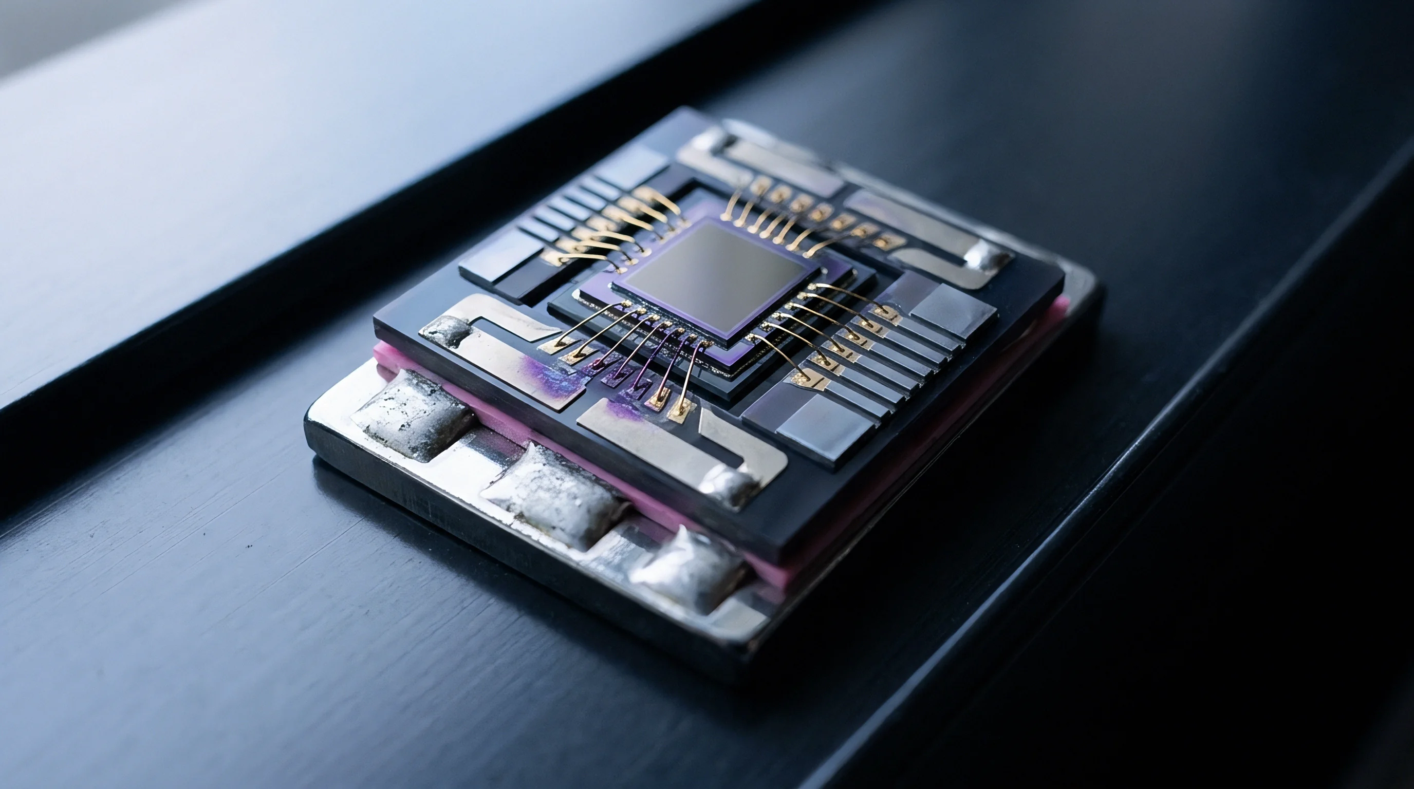
Contractual Allocation of Non-Gaussian Liability
Sourcing agreements that govern microelectronic deliveries replace symmetrical standard deviation metrics with non-parametric quantile limits to establish unambiguous defect boundaries. Master supply agreements mandate clear parametric drift allocation formulas based on baseline test data captured across the manufacturing sequence. When field returns exceed agreed system failure rates, historical baseline differential data identifies which vendor tier introduced the non-Gaussian variance tail.
Financial liability clauses allocate remediation costs proportionally based on decomposed statistical contributions. If mixture modeling demonstrates that OSAT packaging strain relaxation caused 70 percent of recorded tail drift while foundry BTI degradation contributed 30 percent, warranty reimbursement obligations divide along those precise empirical boundaries. Contractual frameworks establish maximum monetary liability caps tied directly to specific parametric quantile limits validated during lot acceptance testing.
Warranty Exposure Modeling for Skewed Drift
Financial exposure calculations for long-life industrial and automotive systems require mapping upper-tail drift probabilities directly to field return cost projections. Standard financial accounting reserves set aside warranty funds based on linear historical return rates. In systems vulnerable to non-Gaussian parametric drift, field returns do not arrive linearly over time.
Heavy-tailed Weibull and Log-Normal degradation curves generate latent failure waves that emerge late in product operating lifespans.
| Specification Strategy | Processing Cost Adder per Unit | Screening Scrap Rate | Unallocated Field Risk Reserve | Primary Contractual Remedy |
|---|---|---|---|---|
| Unconstrained Gaussian (Standard SPC) | Base Pricing ($0.00) | <0.01% at final test | $2.40 per unit deployed | Standard 12-month unit replacement |
| Truncated Quantile Limits (Q0.999) | +$0.18 per unit | 1.2% to 2.5% scrap yield | $0.15 per unit deployed | Tier-proportional cash indemnity |
| Full Non-Gaussian Stress Screening (100% HASS) | +$0.65 per unit | 3.8% to 5.1% scrap yield | <$0.02 per unit deployed | Full warranty reserve rebate & lot reject |
Failure to incorporate non-parametric distribution metrics into master supply agreement indemnity provisions exposes system integrators to unrecoverable field recall costs when long-tail parametric drift triggers widespread system operation breaches.