Forced Air Convective Heat Transfer in Sensor Acceptance Testing
Forced air acceptance testing verifies sensor dynamic response and self-heating limits by replicating application flow velocities and convective coefficients.

Duct
Acceptance testing for temperature elements in airflow channels begins with an unexamined contradiction on the calibration certificate. A factory sheet quotes a thermal response time of 0.8 seconds alongside an accuracy class of plus or minus 0.15 degrees Celsius at zero degrees. That figure comes from an agitated water bath circulating at 0.4 meters per second.
Water transfers heat through liquid contact with a convective coefficient exceeding 1,500 Watts per square meter Kelvin. Place that same six-millimeter sheath inside an ambient air channel moving at three meters per second, and the film coefficient collapses below 60 Watts per square meter Kelvin. The actual response time lengthens beyond twenty seconds.
The incoming lot meets the procurement sheet on paper while failing the dynamic control envelope of the target thermal loop.
Thermal equilibrium in moving gas streams depends directly on the fluid boundary layer clinging to the metallic housing. Still air exhibits thermal conductivities near 0.026 Watts per meter Kelvin, acting as a blanket that resists thermal exchange between the sensor envelope and the primary gas flow. Inducing forced movement strips away this insulating film, raising the local Nusselt number and driving energy into the sensing element.
Testing laboratories frequently run dry calibration checks inside closed ovens with static air or minimal natural convection. Stagnant gas traps heat. Under those static conditions, internal heat generation produces large measurement offsets, while dynamic response curves remain completely unverified.
A six-millimeter probe operating in dry air at five meters per second exhibits a convective coefficient of seventy-two Watts per square meter Kelvin compared to two thousand one hundred Watts per square meter Kelvin in agitated water.
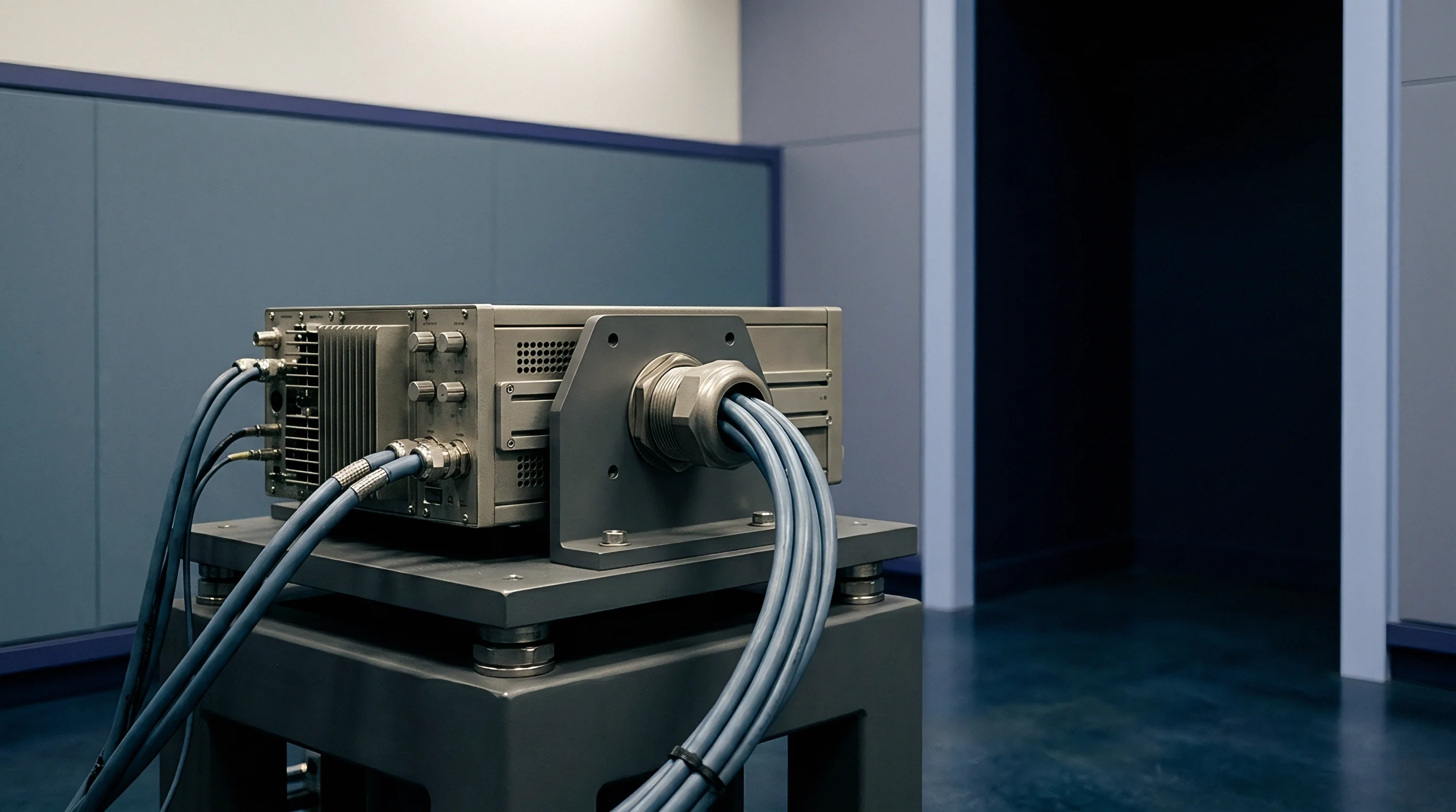
Acceptance rigs demand calibrated wind tunnels capable of delivering steady velocity profiles across the complete test chamber cross-section. Velocity variance across the mounting plane introduces direct measurement ambiguity into the response calculation. Placing reference sensors upstream risks shed vortex interference, while downstream positioning places references in the thermal wake of the unit undergoing evaluation.
Metrology benches resolve this geometry by mounting the test article and reference platinum resistance standards in parallel positions across the uniform core of the channel, perpendicular to the incoming streamline.

Aerodynamic Setup Standards for Gas Calibration
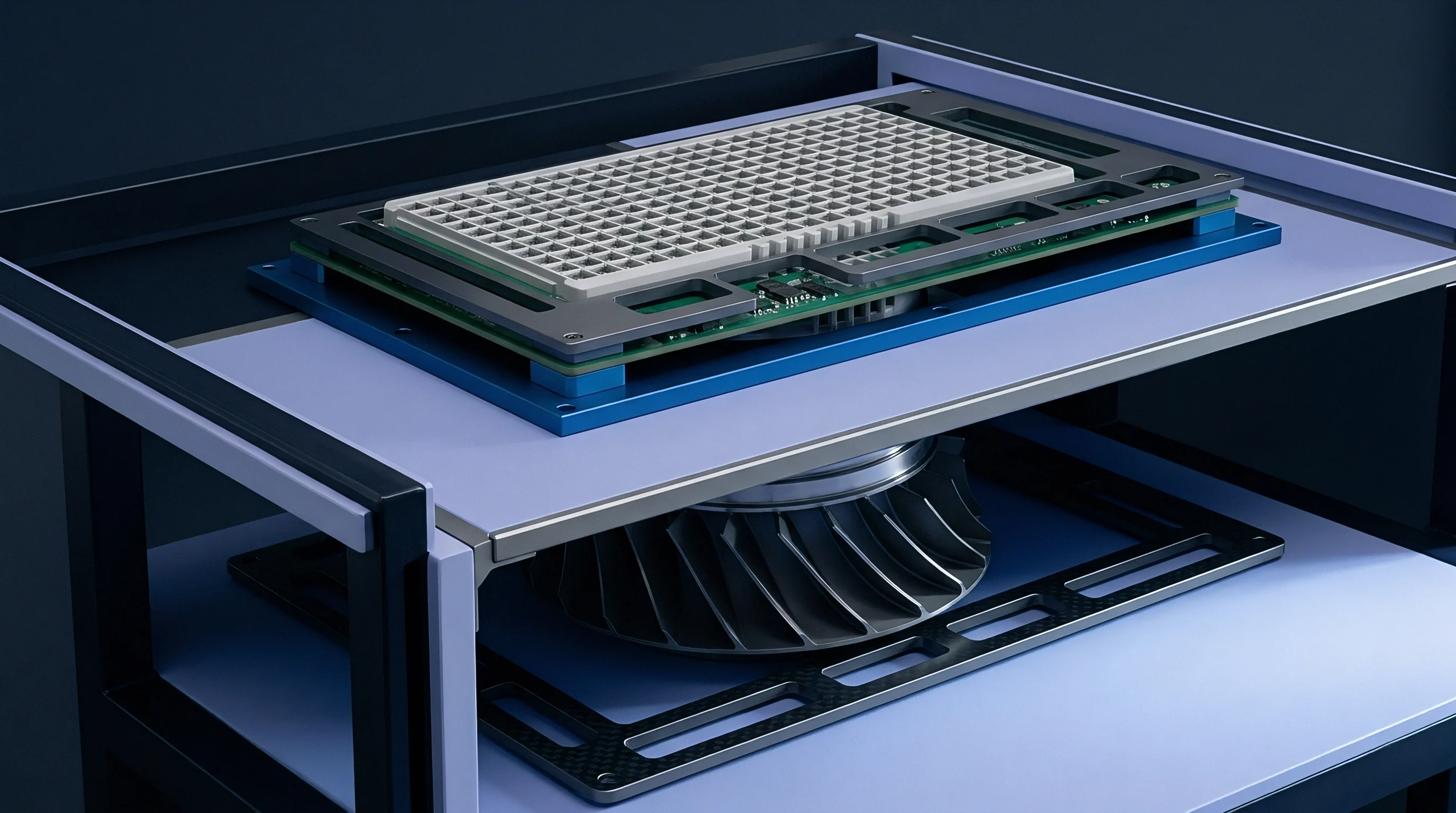
Tunnel construction dictates the repeatability of every dynamic parameter captured during incoming acceptance checks. Straightening vanes upstream of the contraction cone suppress swirling components generated by the blower intake, aligning the flow vectors along the axial coordinate. The contraction zone accelerates the air into the test throat, flattening the mean velocity profile and dropping the freestream turbulence intensity.
Free stream turbulence alters the stagnation point Nusselt number, meaning two tunnels operating at identical bulk velocities produce disparate heat transfer rates if their intake turbulence grids differ. Calibrated hot-wire anemometers map the throat cross-section before sensor insertion, certifying that local velocity across the sensor envelope remains within two percent of the nominal test point.
Tunnel walls introduce boundary layers that grow thicker along the flow direction. Inserting a sensor sheath close to the tunnel boundary exposes the active element to a shear gradient where velocity drops toward zero at the wall. The active portion of an industrial resistance thermometer typically occupies the bottom ten to twenty millimeters of the probe tip.
Centerline immersion positions this active zone within the uniform core flow, preventing boundary layer deceleration from artificially suppressing the measured convective coefficient. Mounting flanges require thermal insulation from the duct shell to stop external duct skin temperatures from conducting down the probe stem to the sensing resistor.
Fluid Discrepancies between Water and Moving Air
Thermophysical properties of dry gas establish a severe barrier to rapid thermal equilibration. Dry air possesses a volumetric heat capacity approximately four thousand times lower than liquid water. Transferring a single Joule of thermal energy from the stream into the protective sheath demands a vastly greater volume of fluid passing across the metallic surface.
The resulting convective heat transfer coefficient scales with the Reynolds number raised to an empirical exponent near 0.6 in transverse flow. The consequence appears immediately on the calibration bench: response rates in gas streams remain sluggish across all standard industrial velocities.
Suppliers avoid testing in forced gas because certified air wind tunnels cost significantly more to construct, operate, and calibrate than standard stirred liquid baths. Liquid immersion tanks deliver rapid stabilization, low spatial gradients, and convenient reference thermometer tracking. Those bath certificates attest solely to the metallurgical purity and base resistance of the platinum wire at thermal equilibrium.
Dynamic parameters, time constants, and self-heating tolerances in gas remain entirely unverified by liquid testing. Specifying incoming verification under ASTM E644 Section 11 forces the vendor to execute dynamic time-constant determinations in air flowing at three meters per second, converting an unverified liquid claim into an enforceable contractual delivery gate.

Boundary
Viscous forces slow the incoming gas stream to zero velocity directly at the sheath exterior, creating the velocity gradient known as the hydrodynamic boundary layer. Concurrent with this momentum drop, a thermal boundary layer forms wherever a temperature difference exists between the gas stream and the thermometer housing. The ratio of momentum diffusivity to thermal diffusivity, expressed by the Prandtl number, sits near 0.71 for air across typical industrial operating ranges.
The thermal boundary layer extends slightly beyond the hydrodynamic layer, presenting a measurable conduction path through relatively motionless gas before reaching the bulk flow.
Air speed dictates response. As velocity increases, aerodynamic drag compresses the boundary layer thickness against the forward stagnation line of the cylinder. The thinning layer reduces the conductive path through stagnant fluid, raising the local heat transfer coefficient.
On the downstream side of the probe, the flow separates, shedding vortices into an unsteady wake where recirculation zones govern heat extraction. The overall heat transfer coefficient represents an integrated average of the thin, high-flux forward stagnation region and the thicker, highly turbulent separation wake.
Section 8 of ASTM E644 binds the supplier to report thermal response times specifically derived in air moving at three meters per second whenever probes target gas ducts.
Acceptance testing quantifies this dynamic behavior through the thermal time constant, tau, defined as the time required for the sensor to indicate 63.2 percent of an applied step change in fluid temperature. The ninety percent response time, t90, equals approximately 2.3 times tau for a first-order thermal system. Industrial probe assemblies deviate from pure first-order models because heat must travel through multiple material interfaces: the outer stainless steel or Inconel sheath, the compacted magnesium oxide insulating powder, and the ceramic substrate carrying the platinum element.
Each layer introduces internal conductive resistance, setting a physical floor below which response time cannot drop regardless of fluid velocity.

What Flow Regimes Alter Sensor Time Constants?
Gas motion across a cylindrical probe transitions through distinct aerodynamic regimes as freestream speed increases from creeping flow to high-velocity exhaust streams. Characterizing these transitions requires calculating the diameter-based Reynolds number across the operating span. Acceptance protocols verify that testing occurs within the specific regime expected in field deployment rather than an arbitrary laboratory setting.
- Creeping Flow occurs below a Reynolds number of four where viscous effects dominate the flow field, producing broad thermal halos and sluggish convective transfer rates.
- Laminar Vortex Shedding emerges between Reynolds numbers of forty and one hundred fifty, generating stable periodic wake structures that produce slight cyclic variations in surface temperature distribution.
- Subcritical Crossflow establishes between Reynolds numbers of one thousand and one hundred thousand, forming thin laminar boundary layers over the nose and turbulent mixing across the detached separation wake.
- Supercritical Flow develops beyond critical Reynolds thresholds where the boundary layer turns fully turbulent prior to separation, dramatically elevating the average Nusselt number across the entire probe circumference.
A probe calibrated at a Reynolds number of two hundred displays an entirely different internal temperature profile than one tested at twenty thousand. The transition shifts the wake detachment point, redistributing the heat flux along the sheath circumference. Acceptance criteria that ignore flow regime allow vendors to quote response figures captured under high Reynolds turbulent cross-flow that field equipment operating in low-velocity exhaust runs cannot reproduce.
Laminar Detachment and Thermal Boundary Layer Resistance
Detachment points on the cylindrical housing dictate the surface area engaged in efficient thermal exchange. Along the forward arc up to approximately eighty degrees from the stagnation line, the laminar boundary layer remains attached, sustaining high temperature gradients into the metal. Past eighty degrees, adverse pressure gradients force the boundary layer to detach from the curvature, leaving a low-pressure wake filled with rotating eddy structures.
The local heat transfer coefficient reaches a distinct minimum near the separation point before recovering slightly within the turbulent recirculation core.
Surface roughness and contamination alter boundary layer detachment locations during operational life. Incoming inspection protocols verify probe surface finish, as coarse machining marks or manufacturing burrs trip the boundary layer prematurely, shifting the local Nusselt distribution. Particulate accumulation during service thickens this boundary layer artificially, adding conductive resistance that mimics thermal drift.
Testing incoming units across multiple airspeeds uncovers whether internal sensor construction or external surface aerodynamics governs the overall thermal impedance path.
Thick boundary layers insulate the probe tip and slow response times under every operating condition.
Velocity
Calibration wind tunnels verify sensor performance by sweeping air speeds across the specified operating envelope while maintaining constant stream temperature. The core mechanism links the convective heat transfer coefficient, h, to fluid velocity through empirical cross-flow correlations. The Hilpert correlation models this relationship as the Nusselt number proportional to the Reynolds number raised to the power m, multiplied by the Prandtl number raised to one third.
For cross-flow past cylinders in typical gas testing ranges, the coefficient C equals 0.683 and the exponent m equals 0.466 for Reynolds numbers between forty and four thousand. At higher velocities between four thousand and forty thousand, C shifts to 0.193 while m rises to 0.618.
The time constant drops. As airspeed climbs, convective resistance at the sheath outer wall decreases, transferring internal conductive resistance to the position of primary thermal bottleneck. Once convective resistance falls well below internal conduction resistance through the magnesium oxide fill, further velocity gains yield diminishing improvements in response time.
A six-millimeter probe experiencing air speeds moving from one meter per second to five meters per second sees its time constant cut by more than half. Increasing velocity from fifteen meters per second to twenty-five meters per second yields less than an eight percent response improvement because internal conduction limits the heat flow rate.
| Medium | Velocity (m/s) | Reynolds Number | Convective Coefficient (W/m²K) | Time Constant Tau (s) | 90% Response Time t90 (s) |
|---|---|---|---|---|---|
| Dry Air | 0.5 | 192 | 28.4 | 38.2 | 87.9 |
| Dry Air | 1.5 | 576 | 46.8 | 24.6 | 56.6 |
| Dry Air | 3.0 | 1,152 | 63.1 | 19.1 | 43.9 |
| Dry Air | 6.0 | 2,304 | 86.7 | 14.8 | 34.0 |
| Dry Air | 12.0 | 4,608 | 124.5 | 11.2 | 25.8 |
| Water | 0.4 | 2,390 | 1,840.0 | 1.4 | 3.2 |
The comparative data exposes the distortion introduced when liquid bath calibration values appear on gas sensor documentation. The time constant in air at three meters per second is more than thirteen times slower than the value achieved in low-velocity water. Acceptance engineers reviewing incoming dossiers verify that test airspeeds match the dynamic requirements of the real duct installation.
The verification sequence requires strict instrumentation controls to prevent aerodynamic artifacts from contaminating the recorded time constants.
Cross-Flow Profiling across the Tunnel Core
Mapping velocity distribution requires pitot-static tubes or calibrated hot-wire probes traversing the duct throat along two orthogonal axes. Acceptance testing mandates that the sensor sheath sits within an isokinetic core where velocity variations remain under plus or minus one percent of the target setpoint. Tunnel blowers generate acoustic pulsations and flow ripples that modulate local boundary layers.
Flow conditioning screens, consisting of woven stainless mesh with forty percent open area ratios, damp out these turbulence pulses when placed in series upstream of the contraction section.
Local shear strips heat. Variations in tunnel temperature during a velocity sweep destroy test validity. Compressing air through a high-pressure blower imparts thermal energy to the fluid, causing bulk tunnel temperature to drift upward during extended acceptance testing runs.
Recirculating wind tunnels require water-cooled heat exchangers positioned downstream of the blower section to lock stream temperature within a tolerance band of plus or minus 0.05 degrees Celsius. Without active thermal stabilization, an apparent sensor step change reflects the drifting background air temperature rather than a pure convective response.
Worked Derivation of Time Constant under Forced Convection
Consider an acceptance evaluation testing a batch of standard Pt100 resistance thermometers housed in six-millimeter outer diameter stainless steel sheaths with a tip wall thickness of 0.5 millimeters. The internal cavity contains compacted magnesium oxide powder surrounding a thin-film platinum element mounted on an aluminum oxide substrate. The incoming inspection specification mandates a response verification in dry air at twenty degrees Celsius moving at a velocity of five meters per second, with an acceptance threshold requiring a time constant tau below sixteen seconds.
Evaluating this assembly begins with the fluid properties of dry air at twenty degrees Celsius and atmospheric pressure: density rho equals 1.204 kilograms per cubic meter, dynamic viscosity mu equals 1.825 times ten to the negative fifth Pascal seconds, thermal conductivity k equals 0.0257 Watts per meter Kelvin, and the Prandtl number Pr equals 0.707. The Reynolds number for cross-flow past the cylinder is calculated directly:
Re = (rho v D) / mu = (1.204 5.0 0.006) / (1.825 10^-5) = 1,979
Using the Hilpert correlation for Reynolds numbers between forty and four thousand, the constants C equals 0.683 and m equals 0.466 yield the average Nusselt number across the sheath circumference:
Nu = C (Re^m) (Pr^(1/3)) = 0.683 (1979^0.466) (0.707^(1/3)) = 0.683 34.12 0.891 = 20.76
From this Nusselt number, the convective heat transfer coefficient h is derived across the outer surface:
h = (Nu k) / D = (20.76 0.0257) / 0.006 = 88.92 W/(m²K)
The total thermal capacitance C_th per unit length of the active sensor tip combines the sheath steel, compacted magnesium oxide, and the central ceramic core. For this specific assembly, material masses and specific heat capacities yield an aggregate thermal capacitance C_th of 10.8 Joules per meter Kelvin across the sensing section. The outer surface area A per unit length for the six-millimeter cylinder equals pi times the diameter, yielding 0.01885 square meters per meter.
External convective thermal resistance R_conv per unit length is calculated as:
R_conv = 1 / (h A) = 1 / (88.92 0.01885) = 0.596 K m/W
Internal conductive resistance R_cond through the stainless wall and magnesium oxide fill adds approximately 0.720 Kelvin meters per Watt between the outer sheath and the internal resistor. Total thermal resistance R_tot equals the sum of external convective and internal conductive components:
R_tot = R_conv + R_cond = 0.596 + 0.720 = 1.316 K m/W
The theoretical thermal time constant tau emerges from the product of total resistance and thermal capacitance:
tau = R_tot C_th = 1.316 10.8 = 14.21 seconds
The calculated value of 14.21 seconds sits safely below the contractual limit of 16.0 seconds. If the laboratory drops the test airspeed to 1.5 meters per second, the convective coefficient falls to 50.8 Watts per square meter Kelvin, pushing external resistance to 1.044 Kelvin meters per Watt and driving tau to 19.05 seconds. A lot accepted at five meters per second fails immediately if tested at 1.5 meters per second.
The physical verification sequence proceeds according to a strict execution path.
- Mount the reference calibrated hot-wire sensor and the test probe in adjacent parallel ports within the wind tunnel test throat.
- Stabilize the tunnel airflow velocity at exactly 5.0 meters per second while running the closed-loop cooling system to hold air temperature at 20.0 degrees Celsius.
- Pre-heat the test probe externally using an isolated radiant shroud until its internal resistance indicates a steady 50.0 degrees Celsius.
- Retract the radiant shroud instantaneously, exposing the probe to the steady cross-flow stream while logging the resistance output at a minimum sample frequency of fifty Hertz.
- Compute the normalized response curve and extract the precise elapsed time corresponding to 38.96 degrees Celsius, representing the 63.2 percent recovery threshold.
Thermal equilibrium takes several minutes. Any deviation in tunnel airspeed during the transition phase alters the local film coefficient mid-test, corrupting the slope of the logarithmic cooling curve. The supplier often asserts that ambient room air testing without forced velocity provides an equivalent baseline for product qualification.

Dissipation
Energizing a resistance temperature detector requires passing an interrogation current through the sensing filament, generating Joule heating equal to I squared times R. This electrical power converts directly to heat inside the platinum element. The sensor must dissipate this internal thermal energy outward through the internal packaging, through the metal sheath, and across the fluid boundary layer into the gas stream. If the dissipation rate is insufficient, the core temperature rises above the surrounding gas temperature, producing a positive measurement offset known as self-heating error.
Convective intensity controls this dissipation mechanism. In still air, where natural convection provides the only cooling path, the dissipation constant of a typical six-millimeter sheath sits between two and five milliwatts per Kelvin of offset. Passing an operating current of five milliamperes through a standard Pt1000 element generates twenty-five milliwatts of internal power, driving an uncorrected self-heating error between five and twelve degrees Celsius.
Increasing the air speed to five meters per second raises the dissipation constant above twenty-five milliwatts per Kelvin, compressing that self-heating offset below one degree Celsius. Acceptance protocols define the test interrogation current alongside the air speed to prevent self-heating from masquerading as calibration offset.
A standard industrial platinum probe tested under stagnant conditions experiences five to ten times greater self-heating bias than the same element tested in a five-meter-per-second air stream.
Stem conduction operates as a secondary, highly destructive dissipation pathway. Heat conducts axially along the sheath wall, the internal lead wires, and the mounting thermowell toward the external pipe wall or duct flange. If the surrounding duct ambient differs from the internal gas temperature, heat leaks along this metallic bridge.
Convective heat transfer from the gas stream must replenish or remove this conducted energy to keep the active tip at true stream temperature. In stagnant or low-velocity air, low convective coefficients fail to counteract axial conduction, driving massive immersion errors.

Self Heating Offsets under Active Airflow
Evaluating self-heating behavior requires running dual-current sweeps at fixed airspeeds within the calibration tunnel. The test engineer records indicated sensor temperature at standard interrogation current, typically one milliampere for a Pt100 element, and then increases the excitation current to two or five milliamperes. The resulting resistance shift reveals the dissipation constant, P_diss, expressed in milliwatts per Kelvin.
Measuring this parameter across airspeeds establishes whether the element maintains internal thermal coupling to the sheath wall.
| Air Velocity (m/s) | Convective Coefficient h (W/m²K) | Dissipation Constant (mW/K) | Self-Heating Offset at 2 mA (mK) | Minimum Immersion Depth (mm) |
|---|---|---|---|---|
| 0.0 (Static) | 8.5 | 3.2 | 125.0 | 145 |
| 1.0 | 38.2 | 14.5 | 27.6 | 72 |
| 3.0 | 63.1 | 23.8 | 16.8 | 56 |
| 5.0 | 88.9 | 31.4 | 12.7 | 48 |
| 10.0 | 118.4 | 42.1 | 9.5 | 41 |
Self-heating inflates indicated values. The tabular data reveals that operating at low velocities severely degrades measurement integrity unless excitation currents are scaled downward. Acceptance testing identifies manufacturing defects such as void formation in the compacted magnesium oxide powder.
An internal air void restricts conductive heat transfer from the platinum coil to the sheath, dropping the dissipation constant and elevating self-heating even when high-velocity air passes over the external metal casing.
Why Do Immersion Errors Escape Initial Bench Checks?
Immersion depth testing uncovers whether convective transfer balances stem conduction losses under field operating velocities. A thermometer inserted into a duct functions as a extended cooling fin. The governing differential equation balances radial convective transfer from the moving gas against axial conduction along the sheath metal.
The temperature distribution along the probe stem follows hyperbolic functions governed by the fin parameter, m_fin, equal to the square root of the convective coefficient times perimeter divided by thermal conductivity times cross-sectional area.
Sheath conduction draws energy outward. When the convective coefficient h is small, m_fin drops, extending the thermal influence of the external cold duct wall deep toward the probe tip. To eliminate conduction errors below 0.05 degrees Celsius, the probe immersion depth must equal at least five to ten times the reciprocal of m_fin.
In a low-velocity air channel of one meter per second, the required immersion depth for a stainless steel sheath reaches seventy-two millimeters. Increasing airspeed to ten meters per second elevates h, compressing the required depth to forty-one millimeters. Factory acceptance checks performed inside shallow test fixtures miss this flaw entirely, delivering sensors that report systematically cold readings once installed in real ductwork.
Deployment of sensors with unverified convective dissipation characteristics leads directly to automated control instability, premature thermal cycling of heating elements, and severe energy waste across industrial air-handling infrastructure.
Settlement
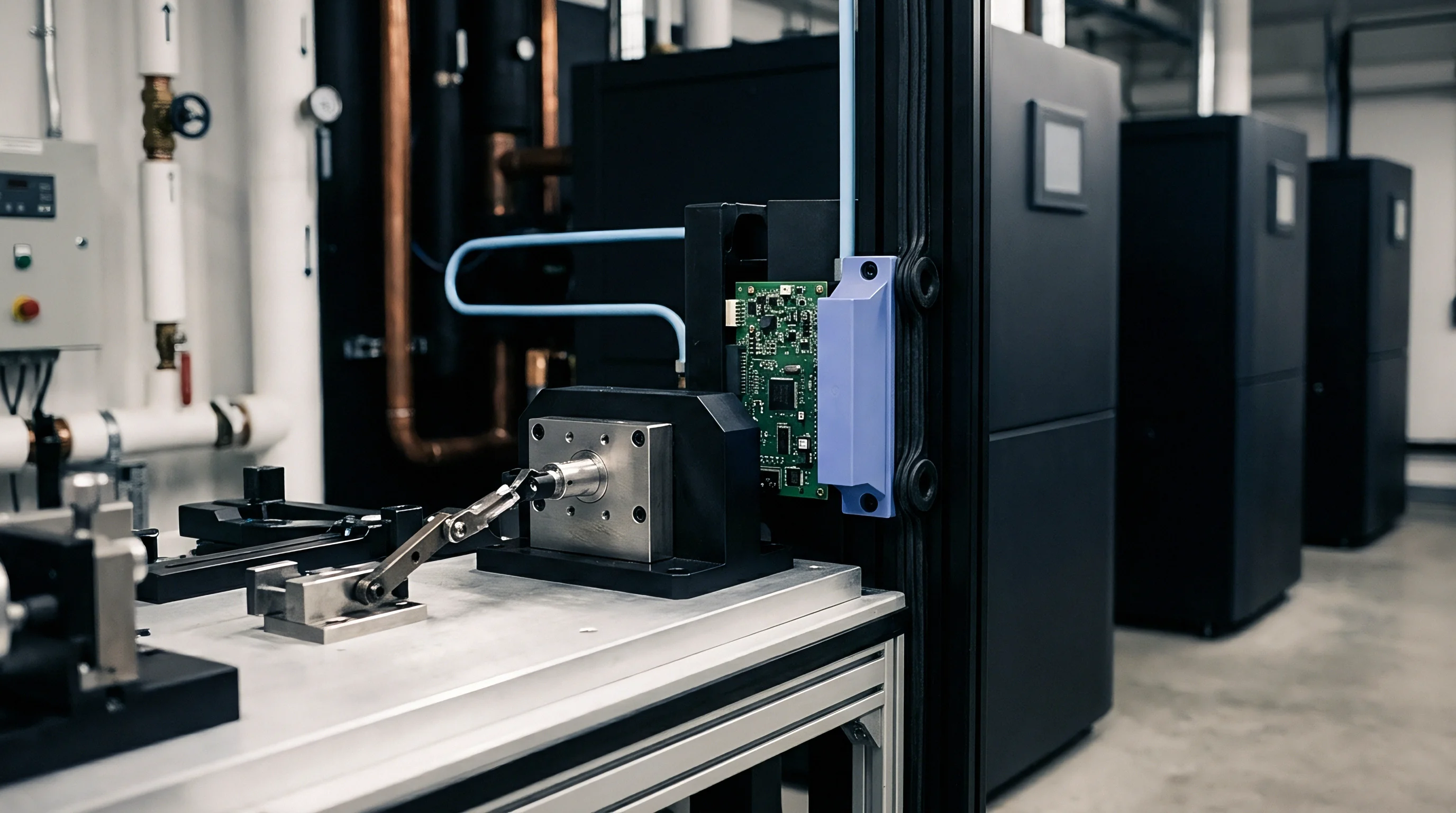
Commercial resolution of sensor performance claims demands clear alignment between the purchase specification and the incoming inspection protocol. When a client rejects an entire incoming lot based on sluggish response or excessive self-heating in air, the supplier routinely points to factory calibration records executed in liquid baths under ISO/IEC 17025 accredited scopes. The accreditation attests to the precision of the electrical resistance measurement and the reference bath stability, but it does not validate sensor dynamics in gas streams.
Without explicit contractual constraints defining the fluid medium, flow velocity, and turbulence intensity for dynamic testing, the buyer holds certificates that are technically valid yet operationally useless.
Buyers absorb the unbudgeted variance. Establishing an airtight procurement dossier requires setting dynamic acceptance limits that account for convective physics. Every purchase order for sensors targeting gas channels must specify the minimum convective dissipation constant and the maximum allowable thermal time constant tau under standardized cross-flow airflow conditions.
Incorporating explicit rejection thresholds protects the buyer from paying sorting costs, engineering rework charges, and delayed commissioning penalties when incoming components fail to track process transients.

Procurement Clauses for Flow Sensitive Calibration Dossiers
A rigorous specification binds the vendor to execute dynamic testing under standardized aerodynamic parameters prior to dispatch. The contract text must explicitly detail the acceptance test apparatus, reference instrument traceability, and flow parameters. Leaving these definitions open invites suppliers to default to cheap, static liquid checks that mask dynamic response failures.
- Aerodynamic Medium Definition requires dry air test streams with relative humidity maintained below forty percent at standard atmospheric pressure to fix gas thermodynamic properties.
- Velocity Envelope Conformance dictates testing at specified nominal flow velocities within an expanded uncertainty of plus or minus two percent, mapped using traceable anemometry.
- Dynamic Step Generation establishes that thermal step changes must be applied via rapid mechanical insertion into a steady cross-flow stream, prohibiting slow thermal ramping.
- Interrogation Current Thresholds mandate that excitation currents during dynamic response logging must remain below one milliampere to isolate convective response from self-heating artifacts.
- Traceable Uncertainty Delivery demands that all reported time constants and dissipation coefficients carry complete uncertainty budgets compiled according to JCGM 100 guidance with a coverage factor of two.
Including these technical requirements in the request for quotation eliminates vendors lacking calibrated aerodynamic facilities before commercial bids are opened. Suppliers with true gas-flow test capability quote prices that reflect the genuine cost of dynamic qualification. The resulting documentation provides legal standing to issue return material authorizations immediately if lot sampling fails incoming wind tunnel checks.

Financial Exposure in Unverified Response Specifications
Procuring temperature instrumentation based strictly on steady-state accuracy claims exposes processing plants to continuous financial drain. In gas turbine inlet monitoring, compressor discharge control, and high-throughput pharmaceutical drying tunnels, dynamic response latency translates directly into over-temperature excursions and wasted thermal energy. A sensor whose response lags by fifteen seconds forces the control loop to widen its safety margin, dropping process operating temperatures and cutting production throughput.
Field retrofits multiply delivery penalties. Replacing hundreds of installed probes across an operational facility costs tenfold more than resolving the specification at the initial procurement stage. The cost of building and maintaining an incoming wind tunnel inspection bench amortizes rapidly across the first rejected lot of non-compliant sensors.
Verifying convective heat transfer performance before parts enter inventory transforms dynamic specifications from marketing claims into verified physical reality.
What remains unsettled is how the industry will standardize aerodynamic turbulence intensity reporting on calibration certificates, given that two tunnels matching in bulk velocity continue to yield diverging dynamic response times on identical sensor geometries.