Lumped Parameter Modeling for Embedded Sensor Thermal Lag Compensation
Lumped RC modeling enables inverse digital filtering in sensor firmware, canceling probe packaging lag to reconstruct fast thermal transients before equilibrium.
Casing
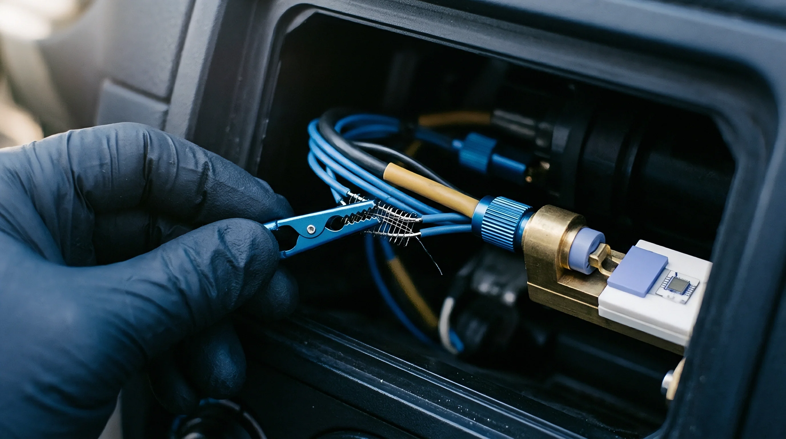
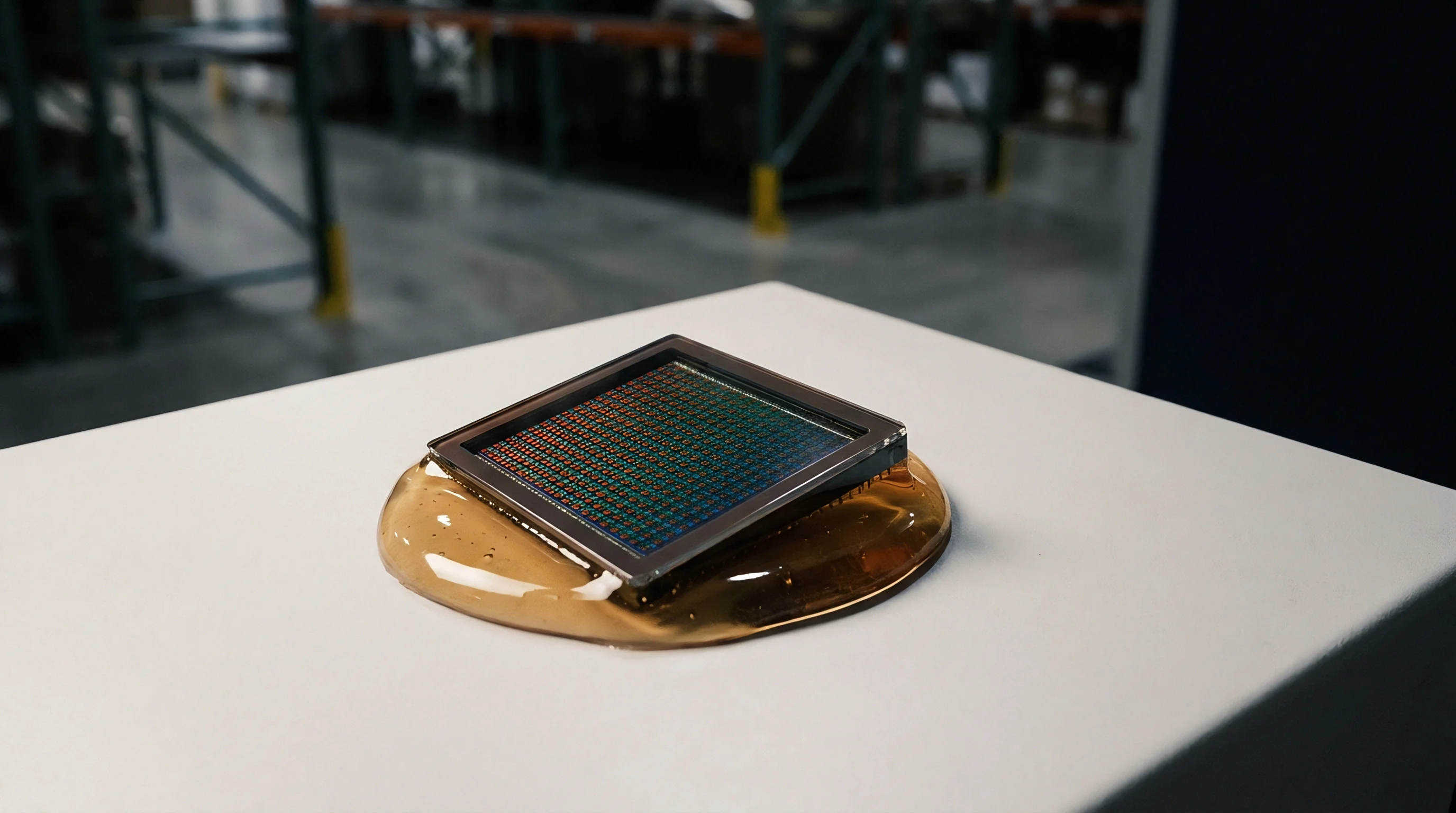
A miniature Pt100 thin-film detector mounted inside a stainless steel probe sheath registers a sudden 40 kelvin step change in fluid temperature with a delay exceeding 1800 milliseconds. Solid packaging layers, potting compounds, internal air gaps, and external fluid boundary layers delay thermal energy penetration. Designers face a structural discrepancy between the environmental medium temperature and the sensing junction reading.
Lumped parameter modeling resolves this discrepancy by mapping physical geometries into discrete thermal resistances and capacitances, generating a digital filter that reconstructs true process conditions in real time before the physical assembly reaches equilibrium.
Silicon exhibits high thermal conductivity. Metal sheaths and protective wells provide mechanical durability and pressure containment while simultaneously acting as low-pass thermal filters. Calculating the Biot number establishes whether internal temperature gradients remain negligible during rapid transients.
When the Biot number remains below 0.1, the internal conductive resistance of the metallic sleeve and inner detector assembly is small relative to the external convective resistance of the fluid boundary layer. Under this condition, treating the entire sensor body as an isothermal node with a single lumped heat capacity introduces less than five percent modeling error.
Packaging mass shifts the measurement phase angle and attenuates high-frequency process fluctuations.
Calculating the Biot number relies on three physical dimensions: the convective heat transfer coefficient of the medium, the characteristic conduction length of the protective enclosure, and the bulk thermal conductivity of the constituent sheath material. When fluid velocity drops, the convective transfer coefficient falls, shifting the primary thermal resistance from the solid shell out into the fluid boundary layer. Conversely, in high-velocity liquid conduits, the convective resistance collapses, and internal conductive resistance through potting resins and ceramic substrates dictates the overall time constant.
Convective Boundary Layers and Biot Criteria
External flow conditions govern heat penetration rates into embedded instrumentation. In oil or water flows exceeding two meters per second, boundary layer thermal resistance drops toward zero, leaving the internal insulation as the dominant impedance. In stagnant air or low-velocity gases, the boundary layer resistance increases by two orders of magnitude, extending sensor response times from hundreds of milliseconds to tens of seconds.
- Air void formation during epoxy potting increases interface thermal resistance by three orders of magnitude over standard polymer conductivity.
- Sheath stem conduction pulls thermal energy along the outer metallic tube into ambient mounting fixtures, establishing permanent measurement offsets.
- Boundary layer stagnation around thick sensor wells suppresses convective transfer coefficients below forty watts per square meter-kelvin in low-velocity gas flows.
- Lead wire dissipation bleeds sensor junction heat directly into copper routing traces on adjacent printed circuit boards.
The junction reaches thermal equilibrium slowly. Packaging geometry dictates transient tracking capabilities long before digital signal conditioning stages process the voltage output. Treating an encapsulated probe as a zero-delay temperature source produces severe closed-loop instability in thermal management firmware, leading to uncorrected excursion events and accelerated battery cell degradation.

Circuit
Thermal transport equations share exact mathematical equivalence with electrical charge networks. Heat flow rate corresponds to electrical current, temperature differential corresponds to voltage, thermal resistance represents the ratio of temperature drop to heat flow, and thermal capacitance represents heat storage per unit temperature change. Formulating a lumped parameter network involves discretizing the sensor probe into localized nodes connected by conduction and convection links.
Epoxy fill adds parasitic heat capacity. Single-node representations assign all mass to one capacitor connected to the environment through one resistor. This produces a first-order differential equation with an analytic solution governed by the product of total resistance and total capacitance, defining the system time constant tau.
Real-world sensor assemblies contain multiple distinct physical zones: the outer metallic wall, the potting resin layer, and the inner platinum or silicon sensing element. Multi-node topologies resolve these discrete stages, assigning dedicated resistor-capacitor pairs to each physical layer to capture high-order transient inflections.
Sensor sheaths with high thermal mass require multi-pole transfer functions to prevent overshoot during sudden thermal shocks.
Heat sinks bleed away measurement flux. Copper traces route heat away rapidly. A two-node lumped formulation models the outer tube as node one and the internal detector die as node two.
Conductive heat transfer across the potting resin couples the two nodes, while external convection feeds the outer node from the surrounding fluid. The resulting second-order state equation models the delayed inflection point characteristic of sheathed probes, where the sensing element initially shows zero response to an external step change before initiating an exponential rise.
Nodal Conductance and Thermal Storage
Material properties dictate equivalent network component values. Selecting packaging elements with low volumetric specific heat capacity minimizes storage delay, while maximizing material conductivity accelerates transmission toward the internal element. When potting resins separate the protective shell from the sensing die, thermal conductivity drops from sixteen watts per meter-kelvin in stainless steel down to 0.8 watts per meter-kelvin in standard electronics potting formulations.
| Material | Thermal Conductivity (W/(m·K)) | Specific Heat (J/(kg·K)) | Density (kg/m³) | Thermal Diffusivity (10⁻⁶ m²/s) |
|---|---|---|---|---|
| Stainless Steel 316L | 16.3 | 500 | 8000 | 4.08 |
| Aluminum Oxide Ceramic | 30.0 | 880 | 3900 | 8.74 |
| Thermally Conductive Epoxy | 1.2 | 1100 | 2100 | 0.52 |
| Silicone Potting Gel | 0.2 | 1400 | 1050 | 0.14 |
| Dry Stagnant Air | 0.026 | 1005 | 1.18 | 21.9 |
Mineral insulation slows internal heat transfer. High thermal resistance steepens phase lag. The product of thermal resistance and capacitance across consecutive nodes forms a transmission ladder that attenuates higher-order temperature harmonics.

Do Internal Temperature Gradients Skew Lumped Capacitance?
Spatially distributed temperature gradients within thick metal sleeves violate the uniform temperature assumption required by classical lumped formulation. When a temperature step strikes a heavy industrial thermowell, the exterior wall heats rapidly while the interior bore remains cold, producing a non-linear spatial gradient across the radial thickness. Modeling this behavior with a single lump underestimates early-stage latency and introduces phase errors into high-speed closed-loop controllers.
Thermowell thickness doubles the response lag. Resolving internal gradients requires splitting the solid sheath wall into three or more concentric cylindrical shells. Each shell layer receives an individual thermal capacitance proportional to its volume and an equivalent radial conductive resistance.
This high-order lumped structure mirrors the diffusion partial differential equation, capturing the steep internal wavefront while maintaining ordinary differential equations suitable for embedded microcontroller execution. A sensor placed in stagnant air behaves like a low-pass filter with a cutoff frequency dictated primarily by outer fluid velocity rather than internal die dimensions.


Inversion
Digital reconstruction algorithms process the raw sensing node signal to regenerate the true environmental temperature profile. The physical sensor behaves as a transfer function containing stable continuous-time poles that damp high-frequency inputs. Applying an inverse filter to the digitized data counteracts these physical poles by placing analytical zeros at matching s-plane locations, theoretically restoring an instantaneous, flat frequency response across the target bandwidth.
Sampling rates fix discrete filter stability. Pure inverse filters contain more zeros than poles, yielding non-causal continuous transfer functions that differentiate incoming signals. To maintain numerical stability and causality in discrete microcontrollers, the inverse formulation incorporates high-frequency parasitic poles located outside the target measurement bandwidth.
These additional poles roll off the compensator gain at elevated frequencies, preventing infinite magnification of high-frequency disturbance terms.
A compensation filter tuned to cancel a 2.4 second time constant amplifies sensor noise by eighteen decibels across frequencies above five hertz.
The Biot number drops below 0.05. Transforming the continuous compensator into discrete time employs the bilinear Tustin transformation. This maps the s-plane transfer function into the z-domain, generating a set of recursive difference equations that execute inside fixed-interval timer interrupts.
The execution cost scales directly with the lumped model order: a single-node compensator requires three floating-point multiply-accumulate operations per sample, while a two-node compensator requires five operations per sample.

Noise Magnification and Regularisation Boundaries
Differentiating incoming measurement signals amplifies broadband Johnson noise and analog-to-digital quantization steps. Because the physical housing attenuates genuine temperature transients at twenty decibels per decade for a single pole, an inverse filter must apply twenty decibels per decade of positive gain across the same spectrum. Without careful regularisation, high-frequency quantization noise swamps the reconstructed temperature signal, causing erratic actuator cycling.
- State equation formulation defines the mathematical relation between sheath temperature nodes and measured sensor junction voltages.
- Continuous pole evaluation extracts natural thermal time constants from step response decay curves.
- Discrete bilinear mapping transforms the continuous inverse compensator into programmable recursive difference equations.
- High frequency pole insertion caps noise magnification at eight times the baseline analogue noise floor to preserve signal integrity.
Analog filtering precedes digital reconstruction algorithms. Gold bonding wires introduce negligible capacitance. Placing an analog second-order Sallen-Key low-pass filter prior to the analog-to-digital converter eliminates out-of-band spectral content that would otherwise fold back into the compensated passband through aliasing.

Is Real Time Numerical Differentiation Stable under Noise?
Numerical instability arises when input noise frequencies coincide with the upward-sloping gain curve of the inverse compensator. A direct inverse filter applied to an unconditioned thermocouple signal produces extreme digital variance, rendering derivative control terms unusable. Deploying a Kalman estimator or a Luenberger observer based on the lumped state equations provides stable state estimates by balancing process model confidence against real-time measurement uncertainty.
The discrete pole shifts toward unity. The state-space observer structure treats the actual environmental temperature as an unmeasured disturbance state, driving internal node models with the estimation error between predicted and measured sensor values. Tuning the observer gain matrix adjusts the convergence rate: aggressive gains yield rapid compensation with elevated noise transmission, while conservative gains smooth high-frequency jitter at the expense of residual thermal phase lag.
Whether dynamic calibration parameters derived under laminar liquid flow maintain valid state estimates during turbulent two-phase boiling regimes remains an open question for embedded firmware designers.

Bench
Empirical extraction of lumped parameters requires controlled thermal excitation in standardized fluid loops. Analytical calculations based on material properties provide starting estimates, but contact resistances between potted components and unpredictable internal air voids create discrepancies between nominal drawings and fabricated hardware. Standard testing protocols plunge the sensor from an isothermal ambient zone into an agitated, constant-temperature liquid bath to generate a near-ideal step input.
Step tests demand rapid fluid immersion. IEC 60751 defines verification standards for industrial platinum resistance thermometers, establishing water bath flow speeds at 0.4 meters per second and air flow speeds at 3.0 meters per second. Water plunge testing isolates internal package conduction by virtually eliminating the external boundary layer resistance, allowing direct measurement of internal resistor-capacitor network values.
Air testing conversely extracts the external convective resistance under known aerodynamic flow.
Compliance with ASTM E644 requires immersion testing in water flowing at 0.4 meters per second, penalizing suppliers who specify thermal response in stagnant air.
The pole shifts toward the origin. Platinum resistance elements follow DIN EN 60751. Recording step responses with a high-speed data acquisition unit reveals the structural order of the sensor assembly.
A purely first-order system exhibits its maximum rate of change immediately at time zero, following a strict negative exponential curve. Sheathed and potted sensors display an initial dead time or inflection zone where the temperature derivative begins near zero, accelerates to a maximum, and then decays, confirming the presence of two or more cascaded thermal nodes.
Transient Response Parameter Extraction
Determining equivalent time constants involves evaluating response markers across the logged step curve. Engineers record the time required to achieve fifty percent of the final step, designated tau-50, and the time required to reach ninety percent, designated tau-90. For an idealized first-order lumped model, the ratio of tau-90 to tau-50 equals 3.32.
When internal thermal capacitance delays heat arrival at the detector, this ratio rises above 4.0, providing an empirical metric to determine whether firmware must instantiate a second-order inverse algorithm.
- Fluid velocity bounds establish the minimum convective coefficient needed to match expected field conditions.
- Immersion depth thresholds prevent stem conduction from draining heat away from the sensing element during calibration plunges.
- Data acquisition sample rate maintains ten samples per anticipated time constant to prevent numerical differentiation aliasing.
Non-linear curve fitting using Levenberg-Marquardt optimization maps recorded plunge data into equivalent multi-node transfer function coefficients. Repeating this extraction across multiple fluid velocities establishes convective resistance as a function of Reynolds number, allowing firmware to scale compensation filter coefficients based on real-time fluid flow measurements. Specifying response time under IEC 60751 Section 6.5 forces the vendor to report separate time values for fifty percent and ninety percent step completions, eliminating single-tau oversimplifications from the procurement dossier.

Procurement
Component selection fixes baseline physical lag before software compensation enters the execution loop. Sourcing decisions balance sensor transduction physics, packaging footprint, mechanical survivability, and manufacturing tolerances. Opting for a heavily sheathed industrial probe simplifies mechanical mounting in high-pressure conduits but imposes severe phase lag that firmware must aggressively invert.
Specifying bare-element thermistors or thin-film platinum chips minimizes physical lag at the cost of vulnerability to chemical attack and mechanical strain.
Raw thermistor curves exhibit severe non-linearity. Negative temperature coefficient thermistors deliver large signal-to-noise ratios, providing high millivolt outputs per kelvin that suppress quantization noise during digital differentiation. Platinum resistance detectors maintain linear calibration across broad temperature spans, simplifying multi-point validation, though their lower base resistance demands precision analog front ends to preserve dynamic resolution.
Bare bead thermocouples offer low thermal mass, achieving time constants below fifty milliseconds in moving water, but introduce cold-junction compensation errors and microvolt-level noise susceptibility.
| Transduction Principle | Typical Time Constant (ms) | Operating Range (°C) | Calibration Tolerance (°C) | Relative Landed Cost |
|---|---|---|---|---|
| Thin-Film Pt100 RTD (Class A) | 1200 to 3500 | -50 to 400 | ±0.15 at 0 °C | High |
| Glass Encapsulated NTC (10k 1%) | 400 to 1800 | -40 to 150 | ±0.20 at 25 °C | Low |
| Exposed Junction Type K | 30 to 150 | -40 to 1100 | ±1.50 or 0.4% | Medium |
| Digital Silicon IC (0402 DFN) | 800 to 2200 | -40 to 125 | ±0.20 at 25 °C | Low |
Supply chain stability varies by sensing modality. Platinum thin-film elements rely on a concentrated tier-one supplier base in Europe and Japan with lead times frequently expanding beyond twenty-six weeks during automotive allocation cycles. Discrete NTC thermistors and standard thermocouples enjoy a broad manufacturing base across multiple global regions, offering shorter lead times and drop-in alternate sources.
Digital silicon temperature sensors combine sensing, reference, and analog-to-digital conversion inside a single surface-mount package, eliminating external signal chain design but locking the embedded firmware into vendor-specific communication registers.
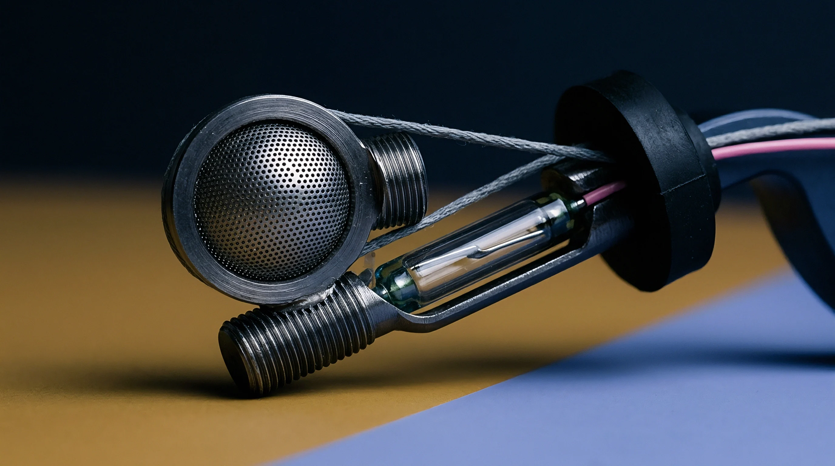
Sensor Modality Selection and Packaging Tradeoffs
Thermal time constants stated on vendor datasheets routinely mislead procurement specifications. Component manufacturers routinely quote response times measured on bare, unpackaged dies plunged into high-velocity water, obscuring the dramatic response degradation that occurs once the die sits inside a protective metal tube backfilled with silicone gel. Procuring engineers establish dynamic performance clauses that mandate testing inside final production housings under minimum expected operational flow velocities.

Supply Base Risks and Vendor Qualification
Vendor batch consistency directly impacts digital inverse filter performance. A compensation algorithm programmed with fixed time-constant coefficients relies on tight physical tolerances during sensor fabrication. When a low-tier supplier introduces variations in potting epoxy volume, shifts internal wire positioning, or alters fill density, the physical time constant drifts across production lots.
This variance causes fixed digital filters to either under-compensate, leaving residual phase lag, or over-compensate, triggering artificial overshoot and ringing in closed-loop controls. Probe manufacturers often assert that custom potting compounds eliminate internal thermal delays, yet factory test reports reveal that mechanical sheath walls dictate nearly all observable lag.