Evaluating Sensor Accuracy Specifications under Ambient Temperature Changes
Sensor accuracy claims established at 23°C fail in service unless temperature coefficients, soak durations, and Total Error Bands are budgeted across the operational envelope.

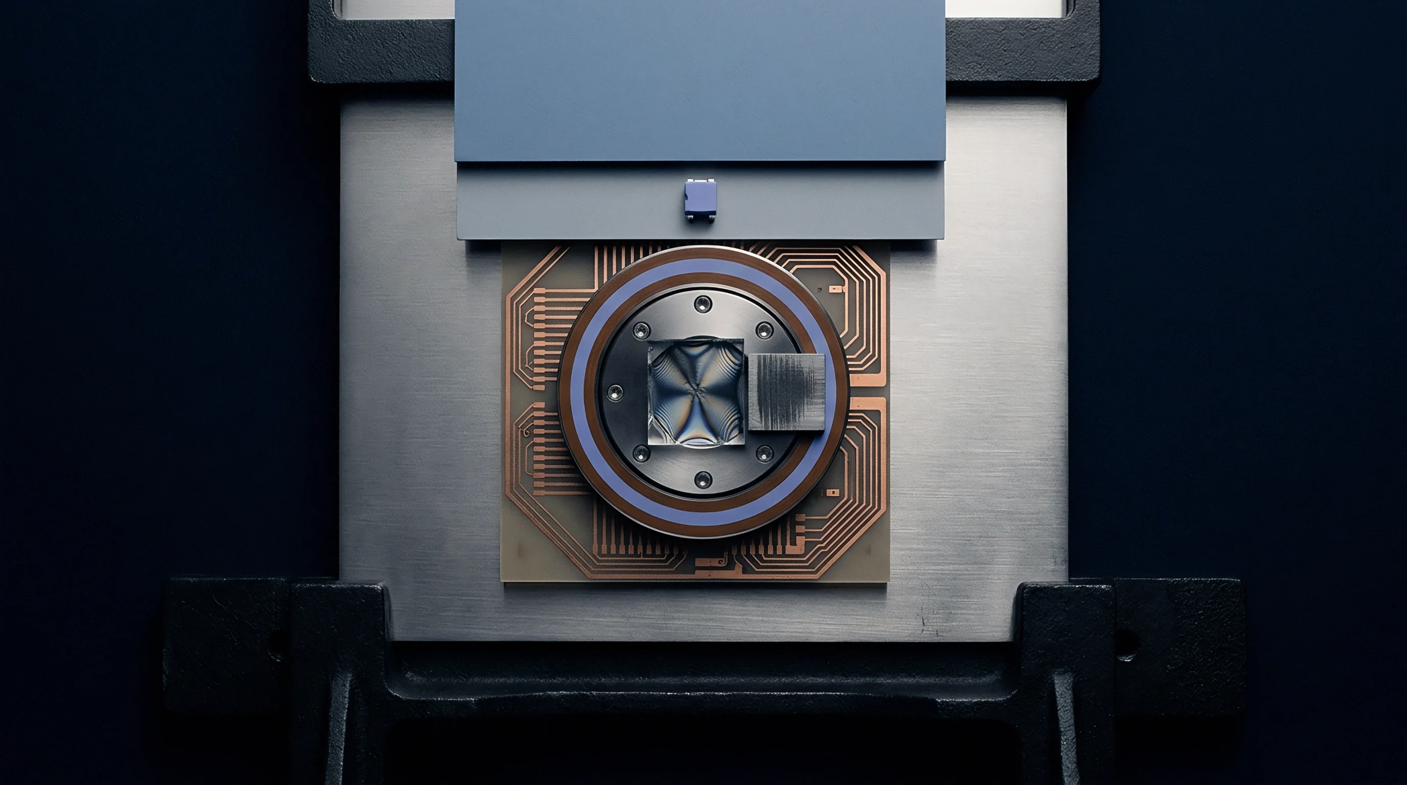
Datum
Sensor specifications routinely highlight accuracy ratings established at 20°C, 22°C, or 25°C under controlled laboratory conditions. Standard room conditions flatter parts. Factory trim fixtures operate within stable ambient environments where humidity sits near 45 percent and convective air movement remains negligible.
Catalogs print reference accuracy figures representing performance at exactly one fixed thermal point. Moving a piezoresistive pressure cell or a thin-film strain element outside that reference point introduces physical reactions that alter mechanical tension, electrical resistance, and semiconductor carrier mobility.
Buyers evaluate these catalog numbers when calculating measurement loops for industrial machinery, exhaust manifolds, refrigeration plants, and remote pipelines. Field hardware experiences diurnal shifts spanning 40°C in outdoor enclosures and process variations exceeding 80°C in engine bays. The catalog figure reflects an idealized operating state.
A transducer certified at plus or minus 0.1 percent of span at 23°C behaves differently when ambient air drops to minus 10°C or climbs to 65°C.
A sensor displaying 0.05 percent span error at 23 degrees Celsius slips to 0.42 percent span error across a 60-degree swing.

Room Temperature Baselines versus Field Envelopes
Ambient exposure alters sensing elements through direct thermal expansion and material property variation. A piezoresistive silicon diaphragm experiences piezoresistive coefficient degradation as temperature rises. Silicon diaphragms stiffen under cold.
Metal film resistors shift resistance based on their intrinsic temperature coefficient of resistance. When ambient conditions deviate from the reference point, three distinct mechanisms degrade output precision: zero shift, span shift, and line-regulation drift.
Piezoresistive pressure transducers document zero temperature coefficients between 0.005 percent and 0.03 percent of full scale per degree Celsius. Temperature changes warp sensor geometry. Over an operational excursion of 50°C, a transducer with an uncompensated coefficient of 0.02 percent per degree Celsius accumulates a 1.0 percent offset shift.
This single temperature-induced error exceeds the base reference accuracy by an order of magnitude. Span shifts add further distortion by altering amplifier gain and sensor sensitivity simultaneously.
| Technology | Reference Accuracy at 23°C | Zero Thermal Coefficient | Span Thermal Coefficient | Operating Span Range |
|---|---|---|---|---|
| Piezoresistive Silicon Pressure | ±0.10% Span | ±0.015% Span/°C | ±0.012% Span/°C | -40°C to 85°C |
| Thin-Film Platinum RTD (Class A) | ±0.15°C | ±0.00385 Ω/Ω/°C | Negligible | -50°C to 200°C |
| Variable Capacitance Ceramic | ±0.25% Span | ±0.008% Span/°C | ±0.010% Span/°C | -20°C to 70°C |
| Foil Strain Gage Diaphragm | ±0.50% Span | ±0.025% Span/°C | ±0.020% Span/°C | -40°C to 105°C |
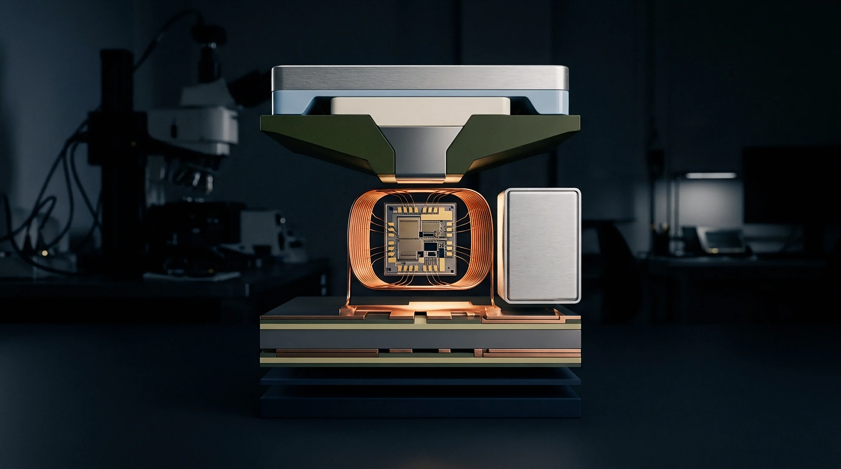
The Anatomy of Laboratory Flattery
Specification sheets separate base accuracy from thermal effects by presenting discrete lines for non-linearity, hysteresis, repeatability, and thermal error coefficients. This division enables marketing documentation to display a headline accuracy of 0.05 percent while burying an additive thermal coefficient of 0.02 percent per degree Celsius in footnote tables. A buyer specifying hardware for a desert pumping station operating between 5°C at dawn and 55°C at noon faces a 50°C ambient spread.
The headline accuracy of 0.05 percent accounts for only one-twentieth of the combined measurement uncertainty.
Manufacturers often test parts in liquid baths or high-velocity recirculating chambers with rapid settling times. These conditions prevent internal heating from compounding external environmental swings. Inside a sealed IP67 industrial junction box, self-heating from excitation voltage traps heat inside the enclosure.
The sensor element sits at 38°C while the outer casing encounters 28°C ambient air. Testing at balanced factory conditions ignores these localized heat traps. Factory representatives routinely claim that laboratory reference figures represent true field capability once ambient swings settle.


Chamber
Controlled environmental enclosures expose transducers to stepped temperature profiles to verify calibration boundaries. Thermal chambers isolate the device from external laboratory drafts and apply convective energy via recirculating blowers. Bench testing without adequate thermal soaking produces misleading results because sensor housings, internal potting materials, and sensing dies exhibit disparate thermal conductivities.
Packaging introduces mechanical stress. An internal silicon die reaches equilibrium at a different pace than a stainless steel 316L threaded housing.
Evaluation programs run through stepped plateaus to identify hysteresis and thermal lag. Rapid temperature cycling without sufficient dwell time causes internal temperature gradients across the sensing bridge. The front face of a diaphragm exposed to the process port registers a different thermal state than the passive compensating resistors positioned on the internal signal conditioning board.
This disparity produces temporary calibration offsets that masquerade as permanent sensor drift.
Heavier sensor housings absorb ambient thermal transients before the internal sensing cell experiences the shift.
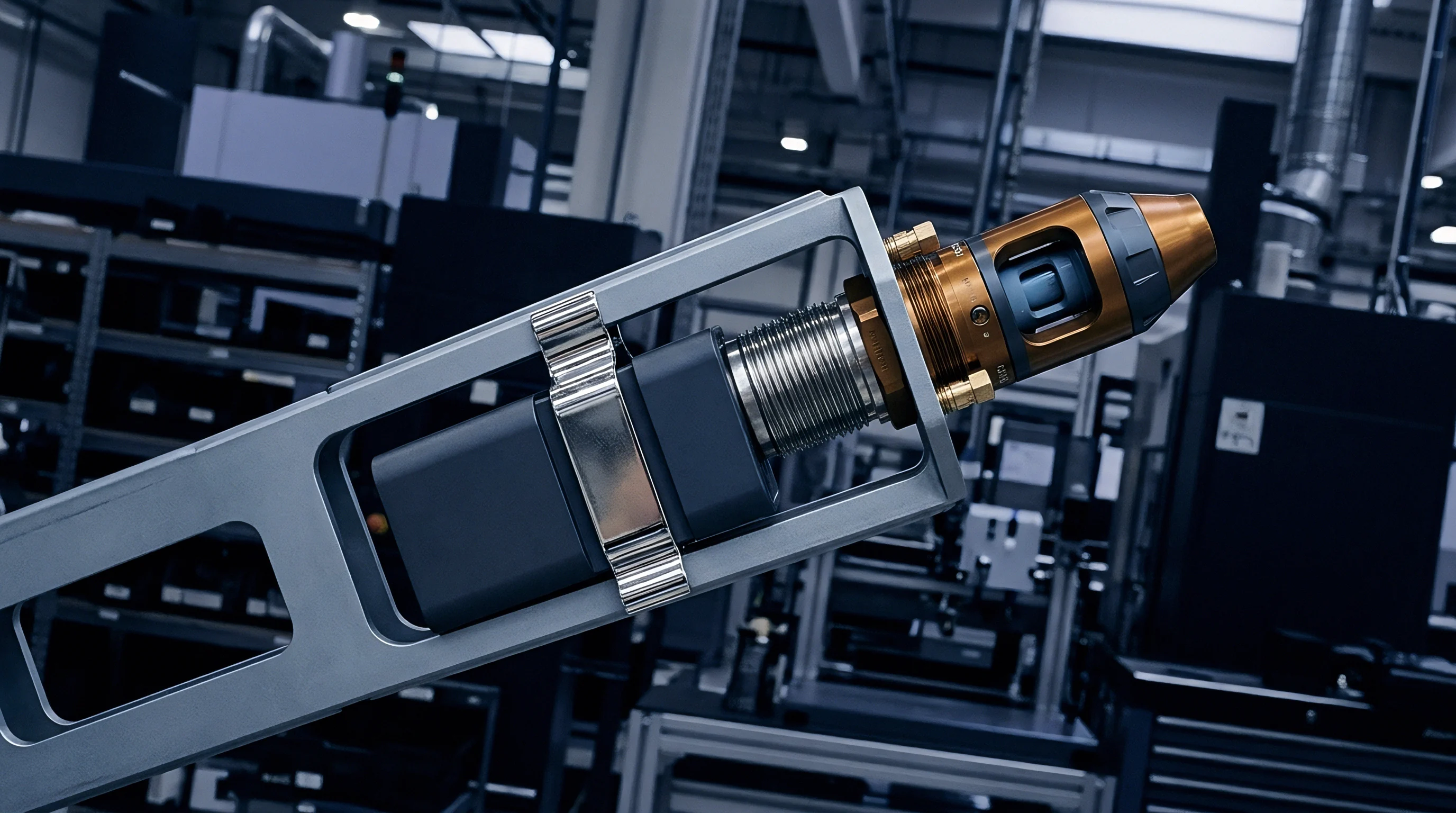
Thermal Mass and Soak Durations
Accurate verification demands precise calculation of thermal time constants for the entire physical assembly. Thermal equilibrium takes hours. A small surface-mount MEMS sensor package possesses a thermal mass under 0.5 grams, allowing thermal equalization within three minutes under forced convection.
An explosion-proof pressure transmitter with an integral terminal housing and thick terminal glass possesses a mass exceeding 1.8 kilograms. Equalizing that assembly across a 40°C step requires an extended soak duration.
The time constant tau defines the period needed for an assembly to achieve 63.2 percent of an applied temperature change in a uniform fluid stream. Five time constants bring the assembly within 0.7 percent of thermal equilibrium with the surrounding environment. For heavy industrial transmitters, tau in still air ranges between 18 and 35 minutes.
An incoming inspection chamber running steps of thirty minutes measures transient thermal lag rather than true steady-state temperature accuracy.

Execution Steps for Thermal Sweep Verification
- Mount the sensor assembly rigidly to an insulated fixture inside the environmental chamber to prevent conductive heat sinking through chamber walls.
- Connect reference excitation power supplies and precision digital multimeters through shielded four-wire cabling rated for the full thermal test range.
- Establish baseline signal output at 23°C reference conditions after a two-hour stabilization soak.
- Ramp chamber temperature to the lowest specified operating limit at a rate not exceeding 2°C per minute to prevent thermal shock in ceramic substrates.
- Maintain the target low-temperature plateau for five calculated time constants based on total transmitter assembly mass.
- Record output zero point and full-scale span values using a calibrated automated pressure or signal generator.
- Ramp the enclosure to the maximum operational rating, repeating the stabilization soak and data acquisition sequence before returning to the 23°C baseline.
Thick aluminum test plates stabilize reading dispersion faster than free air circulation.

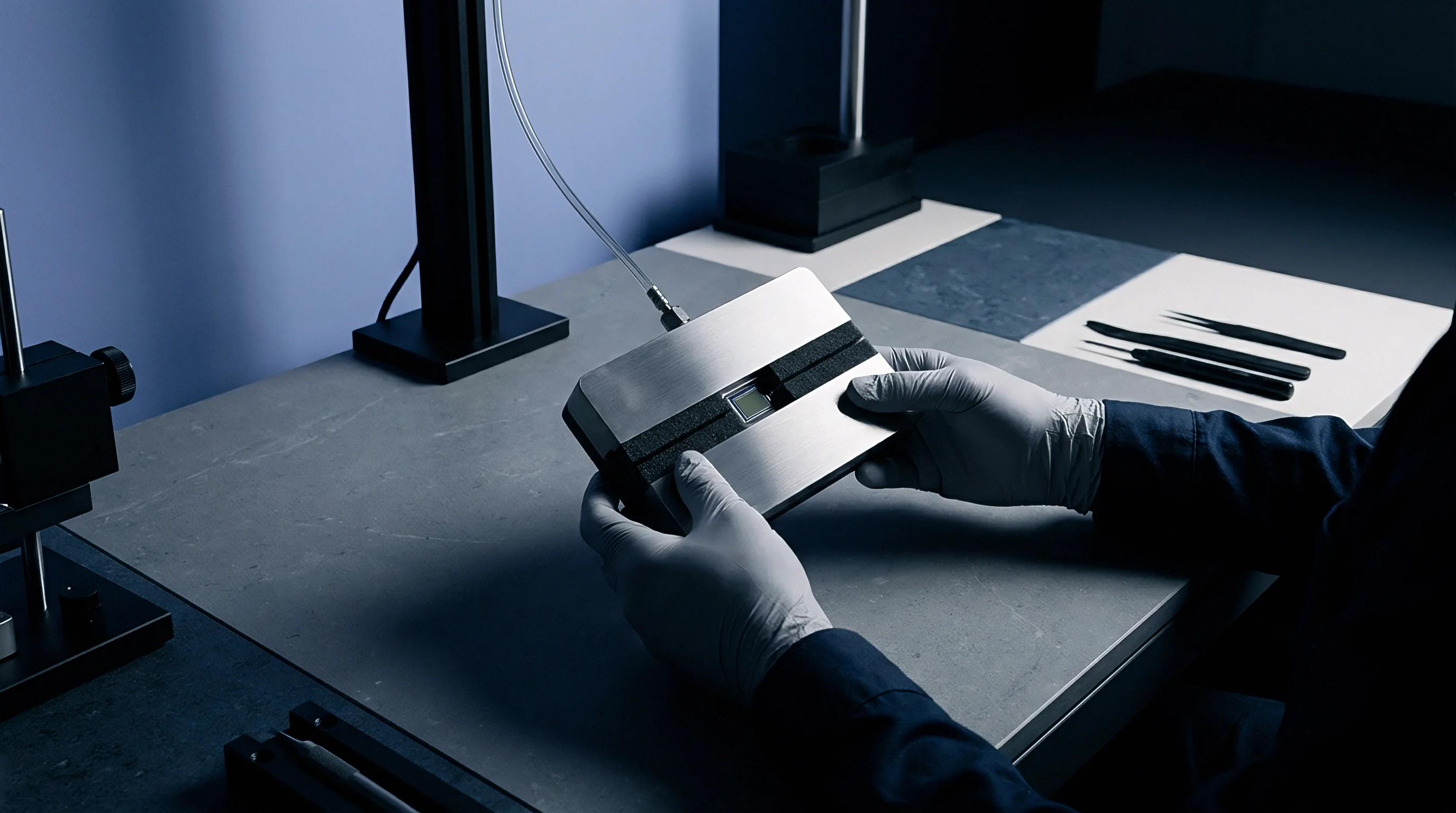
Distortion
Mechanical stress and electrical divergence act simultaneously when temperatures move away from factory calibration baselines. Heat drives fluid expansion. Oil-filled pressure cavities expand against isolation diaphragms, shifting internal pressure distribution.
Transducer components warp at differing rates according to their coefficient of thermal expansion. Silicon has a thermal expansion coefficient around 2.6 parts per million per Kelvin, whereas 304 stainless steel expands at 17.3 parts per million per Kelvin. The adhesive or brazing joint holding the sensor die to the steel header experiences shear force as temperature varies.
This differential expansion introduces mechanical strain into the sensing element that the signal conditioning circuit cannot distinguish from genuine process pressure or mechanical displacement. The induced strain manifests as baseline drift, span attenuation, and non-linear signal curvature. The thermal envelope expands.
Higher temperatures also accelerate leakage currents across semiconductor junctions, degrading signal-to-noise ratios in weak analog outputs.
Thermal hysteresis traps residual mechanical offset after the temperature cycle returns to its starting point.
Where Do Thermal Non-Linearities Compound?
Thermal coefficients rarely remain constant across an operating envelope spanning minus 40°C to 85°C. Uncompensated sensor output follows a parabolic curve across wide thermal spans. The thermal coefficient of sensitivity itself carries a second-order temperature coefficient. Simple two-point analog compensation circuits trim the zero and span errors at room temperature and one elevated point, leaving bow-shaped errors at thermal extremes.
Digital signal processing engines apply polynomial correction algorithms to linearize the temperature response across the full operational range. Calibration rigs capture raw sensor outputs across five or seven discrete temperature points, calculating correction coefficients stored in onboard EEPROM. Inadequate polynomial order leaves residual mathematical ripples across intermediate ranges.
An inflection point between 0°C and 15°C often escapes coarse calibration grids, creating unexpected measurement errors during spring and autumn field operations.

Sensitivity Drift and Zero Shifts
Thermal interference divides into offset changes and scale-factor deviations across operating spans. Zero shift moves the baseline output without altering the proportional response to measured physical inputs. Span shift alters the slope of the calibration curve, multiplying measurement errors as process values climb toward full scale.
- Offset thermal drift moves baseline output uniformly across all measured values through bridge imbalance and asymmetric thermal expansion of packaging materials.
- Sensitivity temperature drift alters output gain through thermal degradation of piezoresistive coefficients or temperature-induced magnetic flux variations in inductive sensors.
- Thermal hysteresis error prevents sensor signals from returning to identical outputs when cycling from hot back to reference versus cold back to reference conditions.
- Thermal transient distortion generates temporary false measurement spikes caused by non-uniform heat transfer across opposing bridge legs during rapid ambient swings.
Misinterpreting temperature coefficients produces unrecoverable systematic measurement drift that invalidates safety limits across three years of operation.

Formulation
Quantifying total sensor error under varying ambient environments involves aggregating multiple distinct uncertainty components into a unified mathematical expression. Uncertainty grows away from datum. The Guide to the Expression of Uncertainty in Measurement dictates methods for combining systematic offsets and random dispersion into expanded uncertainty envelopes.
Combining temperature-induced zero and span shifts with base non-linearity demands rigorous analytical rigor.
Datasheets present accuracy specifications under divergent naming conventions. Manufacturers quote Root Sum Square calculations to market attractive aggregate tolerance bands. Process engineers rely on Total Error Band specifications that aggregate all systematic and thermal deviations into an absolute worst-case envelope.
Understanding the boundary conditions of each calculation separates realistic performance projections from optimistic marketing figures.
Clause 5.3 in standard acceptance agreements penalizes suppliers when thermal non-linearity exceeds stated factory limits.
Root Sum Square versus Total Error Bands
The Root Sum Square approach assumes that individual error sources are completely uncorrelated and distribute normally around a zero mean. Thermal gradients skew internal bridges. The calculation squares each individual uncertainty contribution, sums the squares, and extracts the square root.
Non-linearity, pressure hysteresis, repeatability, zero temperature error, and span temperature error enter the equation as independent terms.
Real-world environmental exposure invalidates the independence assumption underlying Root Sum Square models. Zero drift and span drift originate from identical physical mechanisms: the heating or cooling of the sensing material and its surrounding package. Both errors move simultaneously in response to ambient shifts.
Adding correlated thermal errors using root sum squares underestimates true operational measurement error by 30 to 45 percent. The Total Error Band calculation sums maximum non-linearity, hysteresis, repeatability, and all thermal errors arithmetically over a defined temperature range. This produces an honest boundary that a sensor will not exceed in the field.
| Uncertainty Contribution | Magnitude (% Span) | Probability Distribution | Divisor | Standard Uncertainty (% Span) |
|---|---|---|---|---|
| Reference Non-Linearity (BFSL) | ±0.080% | Rectangular | 1.732 | 0.0462% |
| Terminal Hysteresis and Repeatability | ±0.040% | Rectangular | 1.732 | 0.0231% |
| Thermal Zero Shift (ΔT = 47°C) | ±0.470% | U-shaped | 1.414 | 0.3324% |
| Thermal Span Shift (ΔT = 47°C) | ±0.376% | U-shaped | 1.414 | 0.2659% |
| Calibration Bench Reference Uncertainty | ±0.015% | Normal (k=2) | 2.000 | 0.0075% |
| Combined Standard Uncertainty (Correlated Thermal Components Summed) | 0.6010% | |||

Uncertainty Budget Derivation across Thermal Excursions
Building an uncertainty budget for wide ambient exposures involves a systematic sequence. Assume an industrial pressure transmitter rated 0 to 10 bar, deployed in an outdoor environment spanning minus 20°C to 70°C, referenced to a 23°C laboratory datum. The maximum temperature excursion delta T equals 47°C. The manufacturer quotes a reference accuracy of 0.1 percent, a zero temperature coefficient of 0.01 percent per degree Celsius, and a span temperature coefficient of 0.008 percent per degree Celsius.
Calculating the correlated thermal uncertainty establishes the actual working tolerance. The thermal zero excursion reaches 0.47 percent of span. The thermal span excursion reaches 0.376 percent of span.
Adding these correlated terms produces an aggregate thermal deviation of 0.846 percent. Combining this figure with the base reference uncertainty of 0.08 percent non-linearity and 0.04 percent hysteresis yields an expanded Total Error Band of plus or minus 0.966 percent of full scale across the operating temperature window.
An expanded uncertainty budget incorporates a coverage factor k equals 2 to establish a 95.45 percent level of confidence. When thermal terms receive proper standard uncertainty treatment with appropriate distribution divisors, the resulting uncertainty band guides field instrumentation limits. Field swings expose weak trimming.
Specifying equipment based on unadjusted reference values leads directly to undetected process excursions and out-of-spec products.
Inclusion of IEC 60751 tolerance band extensions across procurement schedules voids supplier warranties whenever ambient exposure exceeds designated thermal boundaries.

Exposure
Long-term field deployment compounds temperature-induced inaccuracies through aging, drift, and cyclic mechanical fatigue. Calibration certificates document past performance. A transmitter that holds its Total Error Band when shipped from the factory drifts as thermal cycles work upon internal solder joints, elastomer seals, and sensor bonding adhesives.
Three years of exposure to seasonal weather cycles induces microscopic structural creep that alters internal stress distributions permanently.
Procurement teams must evaluate not only the initial accuracy across temperature but also the rate of annual calibration drift under thermal stress. High-grade industrial sensors specify long-term stability ratings of 0.1 percent of span per year. In aggressive outdoor installations, repeated thermal cycling between minus 30°C and 60°C accelerates this drift rate by a factor of three.
Ingress protection ratings also degrade over time as elastomeric seals harden under thermal oxidation, allowing ambient moisture to enter the electronics chamber and introduce parasitic resistance paths across high-impedance measurement circuits.

Whose Standard Arbitrates Disputed Field Shifts?
Resolving performance disputes between buyers and manufacturers demands clear contractual alignment on metrological reference standards. Resistance shifts with temperature. International standards IEC 60770-1 and IEC 61298-2 define testing methods for evaluating the effects of ambient temperature on industrial transmitters.
These documents specify ramp rates, soak periods, and error calculation formulas needed to verify compliance.
Contracts that cite simple accuracy percentages without referencing specific testing standards leave measurement disputes legally unresolvable. When an incoming quality audit rejects a sensor shipment based on thermal chamber tests, the manufacturer often challenges the result by citing divergent soak times or alternative pressure reference standards. Clear procurement language establishes the governing test standard, the exact temperature profile, the required stabilization dwell time, and the acceptable uncertainty of the calibration reference equipment.

Procurement Controls for Drifting Sensor Lots
Protecting capital investments against temperature-induced measurement drift involves establishing strict acceptance criteria during the vendor qualification phase. Sensor lots destined for critical monitoring installations must pass thermal screening audits before shipment release. Sourcing agreements should incorporate commercial penalties for units that drift beyond specified Total Error Bands during the initial operational warranty period.
Hysteresis prevents perfect return. Factory calibration certificates must document individual serial number test results at minimum, ambient, and maximum operating temperatures rather than stating generic family conformance. Requiring accredited ISO/IEC 17025 calibration certificates with documented coverage factors ensures that measurement traceability remains intact from the primary reference deadweight tester down to the field device installed on the process pipe.
Whether multi-point thermal compensation justifies tripling initial test expense remains an unresolved commercial debate across high-volume sensor procurement.