Calculating off Diagonal Covariance Terms for Derived Multichannel Measurement Uncertainty Budgets
Off-diagonal covariance terms map shared reference drift and physical cross-talk into derived multichannel uncertainty matrices via Jacobian sensitivity products.
Bridge
Multichannel measurement architecture routinely binds multiple sensor channels to a single physical chassis or shared excitation source. When an array of transducers operates off a common power rail, thermal plane, or mechanical housing, individual channel outputs no longer vary independently. Standard uncertainty budgets that treat each channel as an isolated single-input single-output system miss the structural cross-coupling that dominates derived multichannel vector calculations.
Derived measurement quantities result from combining raw signals across multiple channels through explicit mathematical functions. Examples include calculating total vector force from orthogonal load cells, evaluating spatial temperature gradients from multi-point thermistor arrays, or determining total dynamic power from synchronized voltage and current probes. In each case, calculating the combined standard uncertainty of the derived value requires accounting for both the variance of each individual channel and the mutual covariance between channels.

Common Mode Physical Mechanisms
Excitation voltage drift in an array of strain gauges produces identical proportional shifts across every active channel simultaneously. If the excitation source drifts upward by 0.1 percent, every bridge output scales upward by that same ratio. This creates a strong positive correlation between channels.
Treating these channels as uncorrelated causes significant underestimation or overestimation of derived quantities, depending on whether the derivation involves addition or subtraction.
A shared excitation reference voltage instability of 0.05 percent induces an identical fractional drift across all bridge channels simultaneously, yielding a correlation coefficient of unity between uncorrected channel zero offsets.
Thermal gradients across a multi-sensor enclosure represent another pervasive source of off-diagonal covariance. When ambient temperature swings, thermal expansion and semiconductor resistivity changes alter channel baselines together. Shared excitation alters every output simultaneously.
The magnitude of this correlated drift depends on spatial proximity and material homogeneity across the transducer body.
Common reference standards in laboratory calibration chains also induce mutual correlation among channels calibrated on the same bench. When four thermocouple channels are calibrated against a single reference bath and precision digital multimeter, any systematic error in that reference standard propagates into all four channel calibration factors. The resulting channel uncertainties share a common systematic component that does not average out when channels are summed.

Sensitivity Matrix Coupling Elements
Cross-axis deformation in mechanical transducers creates direct structural interaction between orthogonal measurement axes. Applying a pure axial load along the Z-axis of a multi-axis force platform induces strain in the X-axis and Y-axis sensing elements due to Poisson ratio expansion and mechanical frame deflection. Cross-talk creates systematic output coupling.
Calibrating off-diagonal covariance terms requires isolating these physical cross-sensitivities through structured matrix testing.
Shared signal conditioning circuitry introduces cross-talk through multiplexer charge leakage, ground loop resistance, and board-level parasitic capacitance. High-channel-count data acquisition hardware using multiplexed analog-to-digital converters often exhibits residual charge carrying over from channel N to channel N+1. This dynamic electrical interaction registers as non-zero cross-channel covariance during rapid sampling sequences.
Quantifying these physical linkages relies on separating total channel variance into independent uncorrelated components and shared correlated components. The off-diagonal covariance term between channel i and channel j is calculated as the sum of products of their sensitivity coefficients with respect to each shared influence parameter, multiplied by the variance of that influence parameter. Suppliers often defend uncalibrated cross-talk by claiming that channel isolation specs on datasheets render mutual covariance negligible for routine engineering calculations.
Tensor
Mathematical propagation of multivariate measurement uncertainty relies on linearizing functional relationships around the mean operating point. When output quantities are derived from vector-valued functions of correlated input variables, the covariance structure maps through the transformation via sensitivity matrices. The Guide to the Expression of Uncertainty in Measurement Supplement 2 formalizes this process using linear algebra matrix operations.
Let X represent a vector of N correlated input measurement quantities, characterized by an N-by-N covariance matrix V_X. The diagonal elements of V_X contain the variance of each input quantity, u squared of X_i. The off-diagonal elements contain the covariance terms, Cov of X_i and X_j, defined as the product of the correlation coefficient r of X_i and X_j, the standard uncertainty u of X_i, and the standard uncertainty u of X_j.
Zero correlation represents a rare boundary condition.
Matrix Transformation Architecture
The Guide to the Expression of Uncertainty in Measurement Supplement 2 establishes the linear algebraic propagation framework for vector output quantities. When M derived output quantities Y are calculated from N input quantities X through a set of functional relations Y equals f of X, the combined M-by-M output covariance matrix V_Y is determined by matrix multiplication involving the Jacobian matrix J.
The Jacobian matrix J contains the partial derivatives of each derived output function with respect to each input variable, evaluated at the input vector expectation values. The element in row k and column i represents the partial sensitivity coefficient of output Y_k with respect to input X_i. The total propagation equation takes the form V_Y equals J times V_X times transpose of J. The trace matrix yields derived variance.
| Matrix Component | Symbolic Representation | Mathematical Definition | Physical Metrological Meaning |
|---|---|---|---|
| Input Diagonal Variance | V_X(i,i) | u^2(X_i) | Uncorrelated variance of channel i from random noise and isolated drift |
| Input Off-Diagonal Covariance | V_X(i,j) | r(X_i,X_j) u(X_i) u(X_j) | Mutual covariance between channel i and j from shared influences |
| Jacobian Sensitivity Element | J(k,i) | ∂f_k / ∂X_i | Partial derivative of derived output k with respect to input channel i |
| Derived Output Variance | V_Y(k,k) | u^2(Y_k) | Combined standard variance of derived output metric Y_k |
| Derived Output Covariance | V_Y(k,l) | Cov(Y_k, Y_l) | Propagated mutual covariance between derived outputs Y_k and Y_l |
Direct matrix multiplication scales output variance. Expanding the matrix equation for a single derived scalar quantity Y yields the sum of scaled individual variances plus twice the sum of scaled off-diagonal covariance terms. Ignoring negative off-diagonal terms leads to overestimating total uncertainty, while ignoring positive off-diagonal terms leads to severe underestimation of uncertainty in additive derived channels.
Analytical Decomposition of Shared Influence Quantities
Systematic environmental terms factor directly into individual input variance estimations through partial derivative weighting. When direct measurement of cross-channel correlation coefficients proves difficult, metrologists use analytical decomposition. This technique splits each input channel measurement model into uncorrelated random terms and explicit functional dependencies on shared influence quantities, such as excitation voltage V_ref, ambient temperature T_amb, and calibration standard reference error E_std.
If channel X_1 and channel X_2 both depend on shared influence quantity Z, their off-diagonal covariance is computed by multiplying the partial derivative of X_1 with respect to Z, the partial derivative of X_2 with respect to Z, and the standard variance u squared of Z. Summing these products over all shared influence parameters produces the total off-diagonal covariance input element for V_X without requiring direct simultaneous empirical noise measurement.
ISO/IEC 17025 Clause 7.8.4 mandates reporting individual measurement uncertainties alongside identified covariance components whenever derived multi-parameter values impact conformity statements.
Analytical decomposition eliminates the guessing involved in assigning arbitrary correlation coefficients between 0 and 1. The metrologist identifies physical dependencies, quantifies the variance of each underlying common influence, and evaluates sensitivity derivatives directly from circuit equations or physical laws. ISO/IEC 17025 accreditation scopes for multichannel calibration laboratories require full documentation of these analytical derivative chains whenever cross-channel correlation exceeds 0.1.
Noise
Simultaneous high-speed sampling of parallel analog channels captures transient electrical interference that steady-state models miss completely. Empirical covariance estimation provides a data-driven path to populated covariance matrices when analytical decomposition of circuit physics becomes intractable. Synchronized time-series observations allow direct computation of off-diagonal terms from sampled noise records.
Empirical covariance estimates calculated from finite sample sets introduce statistical variance into the uncertainty budget itself. A small dataset collected during factory acceptance testing may yield sample correlation coefficients that reflect transient bench conditions rather than true population behavior. Sample rate dictates correlation bandwidth.
Why Do Static Correlation Assumptions Fail under Dynamic Thermal Gradients?
Transient temperature distribution changes spatial resistance profiles across sensor arrays at unequal time scales. During rapid thermal cycles, the outer sensors of an array respond immediately to external heat flux, while internal core sensors lag behind due to thermal mass delays. This phase lag causes the cross-channel correlation coefficient to fluctuate in magnitude and invert sign over time.
Static correlation assumptions assume a fixed phase relationship between channels across all operating states. Thermal expansion shifts all strain channels. In dynamic environments, heat conduction equations govern the transient phase shifts, turning static covariance scalar terms into dynamic correlation functions.
Computing uncertainty budgets under dynamic conditions requires applying sliding-window cross-covariance analysis across time-series data gathered during qualification testing.

Empirical Cross-Spectral Covariance Extraction
Time-domain digitizer records provide raw voltage data required to calculate off-diagonal elements directly from sample populations. Given simultaneous N-channel time-series data with K samples per channel, the empirical sample covariance between channel i and channel j is calculated by subtracting their respective sample means, multiplying the residual pairs, and dividing by K minus 1.
- Unsynchronized Sampling Skew shifts time-domain phase alignment between channels, destroying high-frequency empirical cross-correlation accuracy.
- Finite Window Truncation produces high statistical variance in sample covariance estimates when record lengths fall below 1000 samples.
- Quantization Noise Floor masks subtle low-level cross-channel correlation when signal levels occupy fewer than six effective bits of converter range.
- Outlier Voltage Spikes from external electromagnetic interference skew sample covariance values upward, creating artificial correlation terms between unrelated channels.
The calculated covariance matrix fixes the boundary. Spectral analysis provides deeper clarity into frequency-dependent correlation. Fast Fourier Transform processing converts time-domain signals into cross-spectral density functions.
The real part of the cross-spectral density, known as the co-spectrum, isolates co-phase noise components that contribute directly to off-diagonal variance terms, while the imaginary part, or quadrature spectrum, identifies phase-lagged effects that do not alter static sum uncertainties.
Cross-spectral coherence exceeding 0.7 across operational signal bandwidths forces the inclusion of empirical covariance terms in the combined multichannel uncertainty budget.
Uncertainty in the empirical covariance calculation itself follows the Wishart distribution for multivariate normal samples. For a sample size of K observations, the standard uncertainty of an empirical correlation coefficient r near zero is approximately 1 divided by the square root of K. Achieving a 5 percent relative standard uncertainty on an off-diagonal covariance term requires collecting at least 400 synchronized multi-channel samples under stable thermal equilibrium.
When sampling dynamic transient events across a multichannel sensor array, does the empirical covariance matrix maintain positive semi-definiteness during rapid operational state transitions?


Clamp
Demonstrating off-diagonal covariance evaluation requires examining a concrete multi-axis force transducer array operating under shared environmental constraints. Consider a tri-axial force measuring platform designed to evaluate vector thrust in propulsion testing. The platform incorporates three orthogonal bridge channels measuring lateral forces F_x, F_y, and axial force F_z.
The three channels share a common bridge excitation power supply and operate inside an unconditioned environmental enclosure subject to thermal swings.
The engineering objective is calculating the combined standard uncertainty of the total resultant magnitude force vector F_total, defined as the square root of the sum of squared components F_x squared, F_y squared, and F_z squared. Evaluating this budget demands populating both the individual channel variances and the mutual off-diagonal covariance terms between the three force channels.
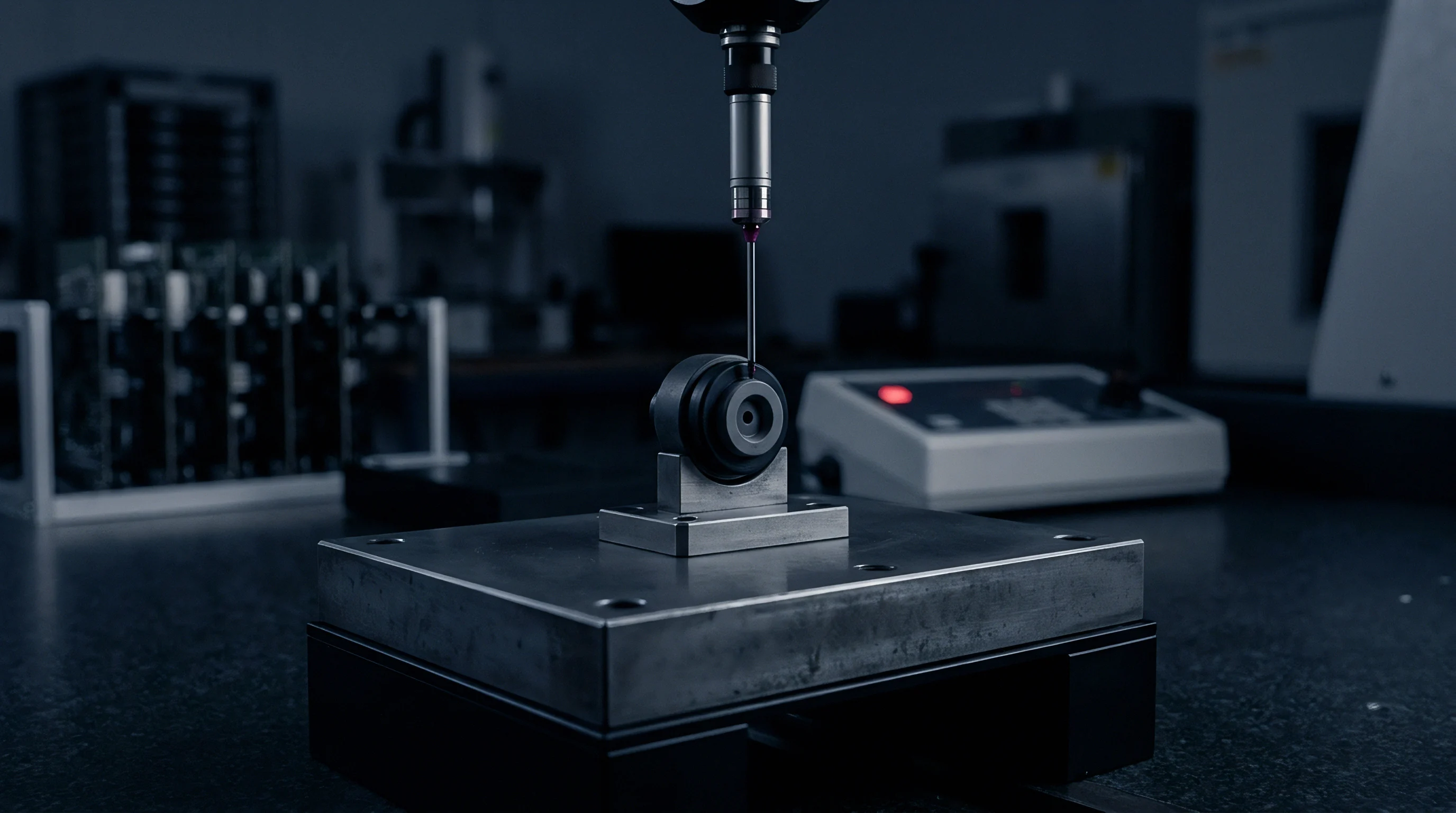
Multichannel Array Calibration Setup
Consider a three-axis load cell measuring orthogonal forces where all three strain bridges receive power from a single precision voltage regulator. Bench characterization under controlled conditions establishes the input channel nominal operating points, standard uncertainties, and physical coupling mechanisms. The measured force components are F_x equals 100.00 Newtons, F_y equals 150.00 Newtons, and F_z equals 500.00 Newtons.
Individual channel uncertainties contain both independent noise terms and correlated systematic terms. The independent standard uncertainties from bridge unbalance and analog noise are u_ind(F_x) equals 0.30 Newtons, u_ind(F_y) equals 0.40 Newtons, and u_ind(F_z) equals 1.00 Newton. The two shared environmental influence factors are excitation voltage instability V_exc with standard uncertainty u(V_exc) equals 0.08 percent relative, and ambient thermal shift Delta_T with standard uncertainty u(Delta_T) equals 3.0 degrees Celsius.
Channel sensitivity to excitation voltage variations is strictly linear: a 1.0 percent shift in V_exc shifts all force readings by 1.0 percent of their nominal value. Channel thermal sensitivities from mechanical frame expansion are c_Tx equals 0.05 Newtons per degree Celsius, c_Ty equals 0.08 Newtons per degree Celsius, and c_Tz equals 0.25 Newtons per degree Celsius.
Explicit Variance and Covariance Calculation Sequence
Evaluating the combined output uncertainty matrix demands systematically computing diagonal input variances alongside mutual correlation terms. First, calculate the systematic uncertainty components resulting from shared influences for each channel.
For channel F_x: the voltage contribution is 100.00 times 0.0008, equaling 0.080 Newtons. The thermal contribution is 0.05 times 3.0, equaling 0.150 Newtons. Combining these with independent noise (0.30 Newtons) via root-sum-squares gives total standard uncertainty u(F_x) equals square root of (0.30 squared + 0.080 squared + 0.150 squared) equals square root of (0.0900 + 0.0064 + 0.0225) equals square root of 0.1189, which equals 0.3448 Newtons.
For channel F_y: the voltage contribution is 150.00 times 0.0008, equaling 0.120 Newtons. The thermal contribution is 0.08 times 3.0, equaling 0.240 Newtons. Combining with independent noise (0.40 Newtons) gives total standard uncertainty u(F_y) equals square root of (0.40 squared + 0.120 squared + 0.240 squared) equals square root of (0.1600 + 0.0144 + 0.0576) equals square root of 0.2320, which equals 0.4817 Newtons.
For channel F_z: the voltage contribution is 500.00 times 0.0008, equaling 0.400 Newtons. The thermal contribution is 0.25 times 3.0, equaling 0.750 Newtons. Combining with independent noise (1.00 Newton) gives total standard uncertainty u(F_z) equals square root of (1.00 squared + 0.400 squared + 0.750 squared) equals square root of (1.0000 + 0.1600 + 0.5625) equals square root of 1.7225, which equals 1.3124 Newtons.
Next, compute the off-diagonal covariance terms using analytical decomposition across the shared influences V_exc and Delta_T.
Covariance between F_x and F_y: Cov(F_x, F_y) equals (partial F_x / partial V_exc partial F_y / partial V_exc u^2(V_exc)) + (partial F_x / partial T partial F_y / partial T u^2(Delta_T)). Substituting values gives (0.080 0.120) + (0.150 0.240) equals 0.0096 + 0.0360 equals 0.0456 Newtons squared.
Covariance between F_x and F_z: Cov(F_x, F_z) equals (0.080 0.400) + (0.150 0.750) equals 0.0320 + 0.1125 equals 0.1445 Newtons squared.
Covariance between F_y and F_z: Cov(F_y, F_z) equals (0.120 0.400) + (0.240 0.750) equals 0.0480 + 0.1800 equals 0.2280 Newtons squared.
| Channel Pair (i, j) | Voltage Covariance Component (N^2) | Thermal Covariance Component (N^2) | Total Covariance Cov(X_i, X_j) (N^2) | Correlation Coefficient r(X_i, X_j) |
|---|---|---|---|---|
| (F_x, F_x) | 0.0064 | 0.0225 | 0.1189 | 1.0000 |
| (F_y, F_y) | 0.0144 | 0.0576 | 0.2320 | 1.0000 |
| (F_z, F_z) | 0.1600 | 0.5625 | 1.7225 | 1.0000 |
| (F_x, F_y) | 0.0096 | 0.0360 | 0.0456 | 0.2745 |
| (F_x, F_z) | 0.0320 | 0.1125 | 0.1445 | 0.3194 |
| (F_y, F_z) | 0.0480 | 0.1800 | 0.2280 | 0.3607 |
Now evaluate the combined uncertainty for the scalar output F_total equals square root of (F_x^2 + F_y^2 + F_z^2). At nominal operating points, F_total equals square root of (100^2 + 150^2 + 500^2) equals square root of (10000 + 22500 + 250000) equals square root of 282500, which equals 531.507 Newtons.
The partial sensitivity derivatives for F_total with respect to each component force are calculated as follows:
c_x equals partial F_total / partial F_x equals F_x / F_total equals 100.00 / 531.507 equals 0.18815.
c_y equals partial F_total / partial F_y equals F_y / F_total equals 150.00 / 531.507 equals 0.28222.
c_z equals partial F_total / partial F_z equals F_z / F_total equals 500.00 / 531.507 equals 0.94072.
Applying the complete law of propagation of uncertainty with off-diagonal terms gives u^2(F_total) equals + 2.
Evaluating the diagonal terms summation: (0.18815^2 0.1189) + (0.28222^2 0.2320) + (0.94072^2 1.7225) equals (0.03540 0.1189) + (0.07965 0.2320) + (0.88495 1.7225) equals 0.00421 + 0.01848 + 1.52433 equals 1.54702 Newtons squared.
Evaluating the off-diagonal covariance cross-terms summation: 2 equals 2 equals 2 equals 0.17706 Newtons squared.
The combined total variance u^2(F_total) equals 1.54702 + 0.17706 equals 1.72408 Newtons squared. Taking the square root yields combined standard uncertainty u(F_total) equals 1.3130 Newtons.
If the off-diagonal covariance terms had been mistakenly omitted, the calculated variance would equal 1.54702 Newtons squared, yielding u_uncorrelated(F_total) equals 1.2438 Newtons. Omitting positive off-diagonal terms understates total measurement uncertainty by 5.3 percent in this specific loading state.
Ignoring positive off-diagonal covariance terms in additive derived functions artificially narrows the calculated combined uncertainty, leading to unearned confidence in marginal calibration data.
Executing an N-channel bench calibration requires a clear systematic protocol to collect and process input covariance structures without missing critical common-mode coupling.
- Mount the multi-channel transducer assembly inside an environmentally controlled calibration chamber with baseline power disabled.
- Connect all channels to the standard target signal conditioning and data acquisition hardware utilizing production cabling setups.
- Apply power and log simultaneous continuous time-series data across all channels for 60 minutes to capture steady-state ambient noise.
- Step the shared excitation voltage supply across its operating tolerance band while recording synchronous multi-channel output steps.
- Ramp chamber ambient temperature across the operational rating window while logging individual channel zero offsets.
- Compute partial derivatives for each channel against excitation and temperature changes using linear regression models.
- Calculate off-diagonal covariance matrix elements by multiplying partial derivative sensitivity pairs by the variance of shared environmental parameters.
- Verify matrix positive semi-definiteness by confirming all eigenvalues of the resulting covariance matrix remain non-negative.
Auditing a multichannel uncertainty budget requires rigorous verification of all supporting physical assumptions and mathematical derivations before accepting stated output tolerances.
- Excitation Isolation Verification confirms whether independent channel power regulators exist or shared rails bind channel outputs together.
- Thermal Gradient Mapping identifies spatial temperature differentials across sensor arrays during transient operational heating cycles.
- Jacobian Derivative Correctness validates partial derivative algebraic formulas against direct numerical perturbation calculations.
- Matrix Eigenvalue Sanity Check ensures calculated covariance structures contain non-negative eigenvalues and valid correlation bounds.
- Reference Standard Traceability Walk traces single calibration standard references shared across multiple channel adjustment chains.
When positive mutual correlation exists between additive channel inputs, calculating combined uncertainty without off-diagonal terms always yields an unrealistically optimistic uncertainty estimate.
Tariff
Ignoring cross-channel correlation terms distorts the multi-dimensional acceptance zone used for pass-fail decisions on complex assemblies. In single-channel testing, conformity evaluation uses a simple interval bounded by upper and lower specification limits. In derived multichannel systems, the specification zone forms an hyper-ellipsoid in vector space whose orientation depends entirely on off-diagonal covariance terms.
When a calibration laboratory evaluates a multi-axis load cell using individual channel tolerances without off-diagonal terms, the declared acceptance region becomes a rectangular box aligned with the coordinate axes. The true confidence region is an elongated ellipsoid tilted at an angle dictated by channel correlation. Parts falling in the corners of the rectangular box pass individual channel checks but fail true vector specification limits.
Acceptance Boundary Contraction
Conformity assessment against multi-parameter specifications requires constructing joint confidence regions that reflect actual channel coupling. Under ISO 14253-1 decision rules, guard-banding contracts the acceptable specification zone by the expanded measurement uncertainty to manage producer and consumer risk. Underestimating covariance distorts these guard bands.
If positive correlation between channels is omitted from the budget, the calculated combined vector uncertainty is artificially small. The guard band applied to the derived output appears narrow, giving the buyer false confidence that the assembly complies with specification limits. Upon deployment in the field, derived vector outputs exceed operational thresholds, generating unexpected customer warranty returns.
| Calibration Coverage Level | Initial Lab Certificate Fee (Relative) | Bench Test Duration Per Unit | False Acceptance Risk Rate | Three-Year Total Landed Cost Impact |
|---|---|---|---|---|
| Uncorrelated Standard (Diagonal Only) | 1.0x (Baseline) | 15 Minutes | 8.5 to 14.2 Percent | High field failure exposure and unbudgeted warranty returns |
| Analytical Decomposition (Shared Inputs) | 1.8x Baseline | 45 Minutes | 1.2 to 2.5 Percent | Balanced commercial cost with predictable field performance |
| Full Empirical Cross-Spectral Covariance | 3.5x Baseline | 180 Minutes | Under 0.1 Percent | High initial testing cost justified for flight-critical hardware |
Overestimating uncertainty inflates hardware build costs. If negative correlation between channels is ignored, the calculated combined uncertainty becomes artificially large. The guard band contracts excessively, forcing the manufacturing plant to reject good multi-axis assemblies that actually fall well within functional limits.
Production yields drop, and unit scrap costs escalate rapidly.
Procurement Terms for Calibration Certificates
Commercial laboratories frequently state channel tolerances individually while leaving cross-channel correlation coefficients unmeasured. Standard accredited calibration certificates based on ISO/IEC 17025 publish scalar uncertainties for Channel 1, Channel 2, and Channel 3 in separate rows of a summary table. They rarely provide the off-diagonal terms necessary to compute derived vector force or power uncertainties.
Uncalculated cross-channel correlations distort the dimensions of the multivariate acceptance envelope and increase true manufacturer risk during acceptance testing.
Procurement teams sourcing multi-channel sensor arrays must explicitly write off-diagonal covariance reporting requirements into supply agreements. Demanding full multivariate calibration certificates adds approximately 80 percent to initial laboratory calibration fees due to the additional thermal and voltage stepping runs required. Contracting for basic individual channel calibration saves upfront laboratory fees while quietly transferring latent quality risk onto the system integration budget.
Underestimating covariance causes unrecorded out-of-tolerance field failures. When derived multichannel accuracy drives safety-critical decisions or high-value fiscal metering, purchasing un-correlated individual channel certificates leaves the system integrator fully liable for uncalculated joint vector errors.