Static Accelerometer Orientation Tumble Calibration Procedures
Static tumble calibration calculates accelerometer bias, scale factor, and cross-axis matrices by optimizing spatial vector residuals against local gravity.

Gravity
Local gravitational acceleration is the primary vector reference for static accelerometer calibration. Because accelerometers measure net specific force, a sensor resting motionless on a rigid surface registers local gravity as a unit vector magnitude. Calculating that local reference accurately is critical.
Baseline surface gravity varies from roughly 9.780 m/s² at the equator to 9.832 m/s² at the poles because of planetary rotation and equatorial bulge. Elevation reduces this value further, dropping roughly 0.3086 m/s² for every thousand meters of height. Defining the reference field at a specific bench requires calculating latitude, altitude, and local density variations through the World Geodetic System 1984 ellipsoidal model alongside free-air and Bouguer corrections.
Precision tilt stages then rotate the sensor’s sensitive axes against this local vertical, projecting known fractions of 1g onto each channel.
Static tumble calibration steps a sensor through discrete, known orientations within this uniform field. Aligning an accelerometer axis directly with the gravity vector yields a full positive or negative 1g reading, while placing it perpendicular gives zero. At intermediate angles, the projected acceleration scales with the cosine of the angle between the sensitive axis and the gravity vector.
The mechanical challenge lies in positioning accuracy: near zero g, the derivative of the cosine curve peaks, making the projection exceptionally sensitive to minor tilt errors. An alignment offset of just 1 milliradian causes roughly 1 mg of error near zero g, whereas that same 1 milliradian offset produces less than 0.5 µg of error when aligned near full 1g.
| Location Identifier | Latitude (Degrees) | Elevation Above Ellipsoid (m) | Theoretical Local g (m/s²) | Standard Uncertainty (m/s²) |
|---|---|---|---|---|
| Equatorial Sea-Level Reference | 0.0000 N | 0.0 | 9.780327 | 0.000005 |
| Taipei Sensing Technology Park | 25.0330 N | 25.0 | 9.789842 | 0.000012 |
| Munich Metrology Center | 48.1375 N | 520.0 | 9.807241 | 0.000008 |
| Eindhoven Integration Laboratory | 51.4416 N | 17.0 | 9.811815 | 0.000010 |
| Polar Metrology Station | 90.0000 N | 0.0 | 9.832186 | 0.000005 |
Field magnitude varies from one facility to another, but stability during testing matters just as much. Structural drift and floor vibrations readily disturb the local vertical reference. Vacuum pumps, HVAC equipment, and foot traffic create micro-seismic noise across the floor, making passive optical tables or pneumatic isolation mounts necessary to filter disturbances above 3 Hz. Unshielded fixtures are also vulnerable to air currents, which cause low-frequency mechanical flutter that mimics bias drift during long static holds.
Shielding the stage inside an acrylic enclosure cuts down these drafts and helps stabilize temperature. Uncontrolled thermal swings expand mechanical mounting fixtures and alter internal sensor die stress, distorting zero-point stability across a multi-position run.
Local gravity maps set the absolute scalar scale factor baseline for every static tumble sequence.
A sensor’s full-scale range determines how much leverage a 1g gravitational standard actually provides. For high-g devices rated to 100g or 500g, tumbling within Earth’s gravity produces very small signal excursions. On a 100g device paired with a 16-bit ADC, a 1g shift covers only 327 counts, leaving calibration coarse; full-range characterization usually requires a centrifuge or dynamic shaker instead.
Conversely, low-g units rated for 2g or 8g span thousands of counts per g. That dynamic range gives tumble routines enough resolution to extract subtle parameters like quadratic non-linearity, cross-axis coupling, and scale-factor asymmetry. In practice, spatial tilt uncertainty remains the dominant error source when solving for zero-g bias.
Thermal gradients inside the package directly distort capacitive, piezoresistive, or optical sensing structures. Power dissipation causes internal self-heating after startup, and rotating the package shifts internal convective air currents across the micro-machined die. In unheated MEMS parts, this thermal redistribution can shift bias by hundreds of micro-g per degree Celsius.
Testing inside an environmental chamber stabilizes these internal micro-gradients and prevents thermal drift from being miscalculated as mechanical non-linearity. Standard procedures require a thermal soak of 15 to 45 minutes at each setpoint before tumbling begins to ensure internal mechanical stresses have relaxed.
Uncorrected tilt errors during these rotations propagate straight into navigation solutions and attitude estimation filters. Similarly, ignoring geographic variations in local gravity introduces a proportional scale-factor error that skews an entire manufacturing run.
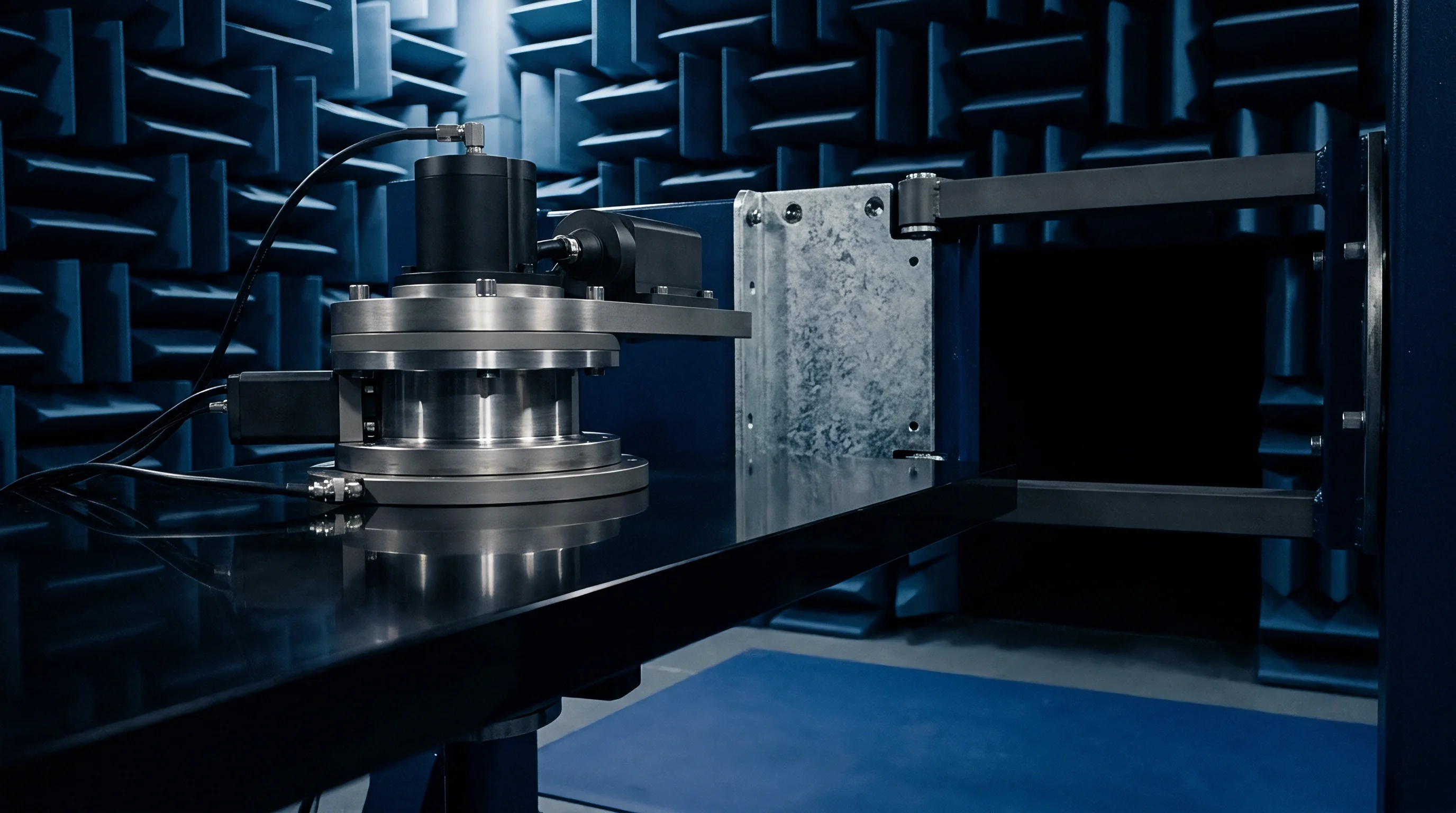
Gimbal
Static orientation calibration depends on rigid, high-precision positioning hardware. Multi-axis dividing heads, rotary tables, and automated gimbals position the sensor at precise tilt and azimuth angles relative to the gravity vector. A two-axis gimbal sweeps the sensor across the unit sphere, orienting sensitive axes toward any coordinate in space, while a three-axis setup provides independent control over pitch, roll, and yaw for redundant verification.
Any spindle runout translates directly into angular error. To maintain accuracy, high-resolution optical encoders mounted directly to the rotation shafts track position to within 2 arcseconds, while mechanical tolerances in the bearings, drive couplings, and gear trains dictate hold-point repeatability.
Aligning the gimbal rotation axes orthogonally to the local gravity vector is essential. Misalignment introduces off-axis tilt during rotation, polluting the reference angles. Electronic autocollimators or dual-axis precision levels are used during initial setup to level the base plate perpendicular to the gravity vector.
Structural deflection is another concern: heavy test fixtures or environmental chambers can cause the gimbal frame to flex as the stage turns. Frame stiffness must keep these structural deflections under 5 arcseconds throughout automated profiles. Direct-drive brushless torque motors are typically preferred over geared systems because eliminating backlash substantially improves bi-directional positioning repeatability.
When qualifying or maintaining a tumble fixture, engineers track several distinct mechanical error sources across the rotation envelope.
- Spindle runout introduces eccentric motion, subjecting the sensor to parasitic linear displacements during rotation.
- Orthogonality error between the primary rotation axes couples motion across axes and corrupts off-axis sensitivity measurements.
- Thermal frame expansion shifts the fixture’s structural center of mass during temperature sweeps, drifting the mechanical zero reference.
- Gearbox backlash creates directional hysteresis whenever a target position is approached from opposing directions.
Production test fixtures use multi-socket carrier nests mounted to a central shaft to balance throughput against structural performance. Fixture design involves a clear tradeoff between thermal mass and mechanical rigidity. High thermal mass slows cycle times because the fixture takes longer to reach equilibrium at each temperature setpoint; low thermal mass risks flexing during rapid indexing moves between hold points.
Hard-anodized aluminum provides a practical balance of stiffness and thermal conductivity for production, while Invar is often chosen for metrology-grade benches where thermal expansion must be kept near zero. Cabling must be handled carefully: power and signal lines should run through low-torque slip rings or loose service loops so cable tension does not torque the stage.
Positioning stages holding two arcsecond angular accuracy preserve sensor noise floor evaluation integrity.
The mechanical interface between the sensor package and the fixture is another common failure point. Surface roughness, particulate contamination, or uneven screw torque will warp the package header. This physical strain transfers into the silicon MEMS die, shifting the zero-g bias and altering scale factors.
Lapping fixture mounting plates to an optical flatness under 1 micrometer prevents this distortion. Technicians use calibrated torque wrenches to ensure uniform clamping across fasteners, though high-volume automated lines often rely on kinematic mounts or custom vacuum chucks to hold packages repeatably without inducing localized stress.
Non-orthogonal alignment between the sensor die and package reference surfaces is the primary contributor to cross-axis sensitivity. If the calibration stage itself has an axis orthogonality error of 0.1 degrees, that mechanical flaw maps directly into the calculated sensor cross-axis matrix. Separating die-level misalignment from stage error requires running a 180-degree tumble reversal.
Flipping the sensor 180 degrees around its measurement axis reverses the gravity vector relative to the die while leaving fixture geometry unchanged, allowing math models to decouple fixture non-orthogonality from internal sensor misalignment.
Automatic software alignment routines cannot fully eliminate the need for mechanical stage leveling during high-precision calibration runs.

Model
Parameter estimation forms the core of static tumble calibration. Linear accelerometer response is modeled through a set of equations accounting for zero-g bias, scale factor scaling, cross-axis coupling, and quadratic non-linearity. This maps the applied physical acceleration vector to the observed sensor output through a formal matrix transformation.
In the linear formulation, the output vector equals a static bias vector added to the product of a three-by-three calibration matrix and the true gravity vector. The diagonal terms of this matrix represent primary scale factors, while the off-diagonal terms capture cross-axis sensitivity and mechanical non-orthogonality. Expanding the equation to capture second-order distortion introduces a quadratic term proportional to the square of the acceleration along each axis.
The complete triaxial model is expressed as:
Y = S M G + B + Q (G ^ 2) + E
Here, Y is the 3×1 vector of measured outputs in volts or raw counts. S is the 3×3 diagonal scale factor matrix. M represents the 3×3 non-orthogonality matrix, configured with unity along the diagonal and cross-axis coupling factors off-diagonal.
G is the 3×1 true gravity vector projected in the fixture frame, and B is the 3×1 zero-g bias vector. Second-order effects are captured in Q, the 3×3 quadratic non-linearity matrix, while E represents residual measurement noise.

Is a Six Position Sequence Adequate for MEMS Accelerometer Calibration?
The number and spatial distribution of tumble positions dictate which error parameters can be solved independently. A standard six-position sequence aligns each axis parallel and anti-parallel to gravity (+X, -X, +Y, -Y, +Z, -Z). This yields six independent scalar equations per axis ~ enough to solve for three zero-g biases and three scale factors.
What it cannot do is separate internal cross-axis coupling from external mounting misalignment, nor can it isolate quadratic non-linearity from scale-factor asymmetry.
Stepping up to a 12-position routine adds face-diagonal orientations where two axes simultaneously experience roughly 0.707g. This provides the cross-axis excitation needed to resolve the off-diagonal terms in matrix M. A 24-position sequence goes further, distributing 45-degree orientations across all spatial quadrants. This broad distribution completely uncouples the quadratic non-linearity terms Q from scale factor S and cross-axis terms M, providing full mathematical observability across the parameter space.
| Tumble Sequence Profile | Total Orientations | Observable Parameters | Bias Uncoupling Quality | Cross-Axis Decoupling Capacity | Non-Linearity Isolation |
|---|---|---|---|---|---|
| Basic Orthogonal Six-Face | 6 | 6 (3 Bias, 3 Scale) | Moderate | Unobservable | Unobservable |
| Face-Diagonal Expanded | 12 | 12 (3 Bias, 3 Scale, 6 Cross) | High | Fully Decoupled | Partial Coupling |
| Symmetrical 24-Position Multi-Axis | 24 | 15 (3 Bias, 3 Scale, 6 Cross, 3 Quad) | Very High | Fully Decoupled | Fully Decoupled |
| Over-Sampled 36-Position Icosahedral | 36 | 15 + Residual Noise Model | Maximum | Fully Decoupled | Fully Decoupled |
Extracting these parameters requires non-linear least-squares optimization over the complete tumble dataset. If the positioning fixture uses calibrated optical encoders, the true gravity vector G is known directly in the stage coordinate frame for every orientation. The objective function then minimizes the sum of squared differences between predicted outputs Y and actual sensor measurements across all N orientations.
When using manual flip blocks lacking angle encoders, the absolute direction of gravity relative to the block faces is unknown. In that scenario, parameter estimation relies on the invariant magnitude of the gravity vector. Because local gravitational magnitude remains constant regardless of spatial orientation, the vector sum of the calibrated outputs must equal local g at every static position.
The scalar magnitude cost function minimizes deviations from this local standard:
Cost = Sum
This scalar invariant approach solves for zero-g bias and scale factors without requiring high-precision stage encoders. The limitation is that it cannot solve for the sensor’s absolute spatial orientation, leaving frame alignment uncalibrated unless at least one axis is referenced externally.
Numerical solvers like Gauss-Newton or Levenberg-Marquardt iteratively refine parameter estimates starting from nominal values. Convergence depends heavily on initial conditions and data noise. If the chosen tumble orientations cluster too closely together, the data matrix becomes ill-conditioned, leading to divergent solutions or noisy cross-axis estimates.
Distributing orientations uniformly across the unit sphere keeps condition numbers low, speeding up convergence and tightening estimation confidence.
Scalar invariant calibration models resolve sensor bias without requiring high-precision angular encoder hardware.
A practical comparison highlights the impact of position counts. Take a capacitive MEMS triaxial accelerometer with a nominal scale factor of 1000 counts per g and a nominal bias of 0 counts. Running this sensor through both a 6-position and a 24-position sequence under identical laboratory conditions demonstrates the difference in parameter resolution.
Processing the 6-position dataset yields an estimated X-axis scale factor of 1004.2 counts/g and a zero-g bias of +14.2 counts. Because the 6-position fit cannot separate higher-order terms, structural non-linearity in the MEMS beam is absorbed directly into the scale factor. In the 24-position sequence, the solver successfully separates these effects: the linear scale factor resolves to 1001.8 counts/g, bias shifts to +12.1 counts, and a quadratic non-linearity of 2.4 counts/g² is extracted cleanly.
Relying strictly on 6-position data masks this second-order behavior, which shows up as scale-factor error when the sensor approaches full scale.
Calibration orientation sequence selection follows sensor performance class expectations.
Residuals
Residual analysis is the primary diagnostic for checking calibration quality. Once the optimization routine converges, predicted outputs are generated for each tumble orientation and subtracted from the raw observations. In a well-behaved calibration free of unmodeled dynamics, these residuals distribute normally around zero mean, bounded only by broad-band sensor noise.
Systematic curvature, clustering, or outliers in residual plots indicate mechanical fixture play, unmodeled sensor non-linearities, or environmental interference during the run.
ADC resolution, sampling frequency, and integration dwell time define the baseline noise floor of the collected tumble points. Raw sensor output contains a mix of thermal noise, 1/f flicker noise, and quantization error. Averaging samples over a stationary dwell window reduces broad-band white noise by the square root of the sample count: sampling at 1000 Hz for 2.5 seconds yields 2500 samples, cutting broad-band noise by a factor of 50.
However, averaging past the sensor’s bias instability point becomes counterproductive, as flicker noise and slow thermal drift begin corrupting the mean.
| Sampling Rate (Hz) | Dwell Time per Position (s) | Total Samples Averaged | ADC Bit Depth | Quantization Noise Floor (µg) | Effective Bias Uncertainty (µg) |
|---|---|---|---|---|---|
| 100 | 0.10 | 10 | 12 Bit | 488.0 | 154.3 |
| 1000 | 0.50 | 500 | 16 Bit | 30.5 | 1.36 |
| 1000 | 2.50 | 2500 | 16 Bit | 30.5 | 0.61 |
| 4000 | 5.00 | 20000 | 24 Bit | 0.12 | 0.08 |
| 4000 | 20.00 | 80000 | 24 Bit | 0.12 | 0.14 |
Allan variance curves determine the practical dwell time for static holds. Plotting Allan deviation against integration time shows distinct noise regimes: the initial negative slope indicates white noise, where averaging actively improves measurement precision. The flat trough marks the sensor’s bias instability floor, representing the practical limit of integration.
Dwell times extending beyond this minimum expose data to random walk drift. For typical capacitive MEMS devices, this minimum falls between 2 seconds and 10 seconds of dwell time.
Data collection routines should enforce a strict sequence during each orientation step to keep mechanical settling transients out of the solver.
- Rotate the gimbal stage to target orientation coordinates at controlled angular velocity to limit mechanical shock.
- Enforce a mechanical settling delay of 1.5 seconds to permit fixture vibration dampening and structural stabilization.
- Verify sensor internal zero-velocity logic states to confirm the absence of residual rotational dynamics.
- Initiate synchronous over-sampled data acquisition across all active sensor channels simultaneously.
- Calculate real-time running variance over the sample window to flag external vibration impulses.
- Compute the mean static vector value and store it alongside encoder spatial coordinate records.
Mechanical settling delays are critical before sampling begins. High-speed stage moves ring the mechanical structure of the gimbal, mounting nests, and internal sensor suspension. In lab testing, settling windows under 800 milliseconds allowed structural vibration to corrupt static averages.
Capacitive and piezoresistive proof masses need brief damping periods to settle within 1 micro-g of rest after indexing. Setting a programmable settling delay guarantees this dynamic ringing decays before data logging starts.
Standard qualification procedures enforce residual root-mean-square limits below 500 micro-g for tactical sensor acceptance.
Thermal time constants also introduce residual errors during multi-point sequences. Repositioning a sensor alters air convection patterns around its housing, and the resulting thermal shifts across the silicon element cause zero-g bias to wander mid-test. This drift shows up as characteristic hysteresis in residual plots when the stage revisits earlier orientations.
Enclosing the stage within a temperature chamber equipped with forced-air circulation stabilizes surface boundary temperatures and eliminates these localized convection transients.
Do residual spatial errors stem from silicon die stress or package-level mechanical distortion?
Audit
Procuring precision accelerometers requires aligning calibration rigor with design requirements. Datasheets frequently list nominal scale factors and bias stabilities derived from single-axis testing or batch sampling. Critical applications ~ such as inertial navigation, bridge health monitoring, and robotics ~ require traceable multi-position calibration datasets for every serialized part.
Procurement documentation should clearly specify orientation counts, temperature points, and acceptable residual limits to keep out-of-spec hardware out of production builds.
Metrology standards give engineering teams a solid baseline for calibration compliance. IEEE 1293 outlines specification and test formats for linear single-axis accelerometers, defining measurement protocols for scale factor, bias, axis alignment, and temperature coefficients. ISO 16063-16 specifies procedures for static calibration using Earth’s gravitational field.
Referencing ISO 16063-16 in vendor purchase agreements establishes unbroken traceability to international metrology standards and provides clear criteria during quality audits.
Procurement teams use a structured audit checklist to verify vendor compliance during incoming lot inspections.
- Traceability dossier linking factory reference standards to recognized national metrology institutes.
- Tumble matrix raw data containing uncorrected output counts across all standard test orientations.
- Residual fit variance metrics confirming mathematical convergence within agreed acceptance limits.
- Environmental logs proving thermal chamber stability within plus or minus 0.5 degrees Celsius throughout testing.
- Rotational stage encoder certificates documenting angular accuracy verification within the preceding 12 months.
Test costs scale directly with the number of tumble positions and thermal dwell cycles. A basic 6-position room-temperature tumble in a production socket adds very little unit cost, but leaves cross-axis coupling and second-order distortion uncharacterized. A full 24-position sequence run across -40°C, +25°C, and +85°C requires environmental chamber time and longer settling holds, driving up test expense significantly.
Selecting the calibration routine is ultimately an economic decision balancing target sensor performance against unit test budgets.
Incoming qualification should evaluate residual error distributions rather than trusting nominal datasheet values. Automated vendor test stations can report misleadingly low residuals if their optimization routines are under-constrained. Requiring vendors to supply raw, uncorrected tumble vectors alongside final matrices allows receiving teams to rerun least-squares fits independently, catching artificial constraints, faulty assumptions, or aggressive outlier filtering in factory test code.
Standard procurement contract terms require suppliers to provide automated tumble verification dossiers containing uncorrected spatial raw data vectors for every calibrated sensor lot.