Allan Variance Identified Parameter Translation into Discrete Kalman Filter Covariance Matrices
Allan variance parameters translate into discrete Kalman covariance matrices by integrating continuous spectral densities scaled by sample interval durations.
Extraction
Stationary data collected from a single-axis vibratory rate gyroscope over thirty-six hours at a constant 25 °C reveals an uncompensated zero-rate drift of 4.2 millidegrees per second. Plotting the two-sample Allan deviation against cluster averaging time τ on logarithmic axes maps distinct physical phenomena to characteristic linear gradients. White noise yields slope minus one-half.
Short averaging clusters expose high-frequency broadband readout electronics and capacitive transducer thermo-mechanical Brownian motion, whereas wide averaging intervals unmask long-term thermal gradients and material stress relaxation in the micromachined suspension beams.
Identifying the precise coefficients requires locating specific averaging points along the Allan deviation curve σ(τ). The Angle Random Walk coefficient N, expressing angular rate white noise, equals the value of σ(τ) evaluated directly at τ = 1 second, expressed in units of degrees per square-root hour or degrees per second per square-root Hertz. When examining the positive slope region where σ(τ) scales proportionally with τ^(+1/2), the Rate Random Walk coefficient K maps directly to the value of σ(τ) at τ = 3 seconds.
The lowest stationary point on the trace represents the bias instability plateau, where 1/f flicker noise dominates sensor output before environmental fluctuations force the trajectory upward into rate ramps.
A flat noise floor masks underlying thermo-mechanical brownian motion across narrow integration windows.
The mathematical correspondence between Allan deviation parameters and continuous stochastic processes follows strict linear relations:
- Quantization noise creates a log-log slope of minus one at short cluster intervals, governed by analog-to-digital converter bit width and decimation register architectures.
- Angle random walk establishes a slope of minus one-half across mid-frequency bands, originating from thermomechanical dissipation inside the micromachined resonator cavity.
- Bias instability produces a zero-slope plateau at intermediate averaging intervals, generated by flicker noise in sense amplifier transistor channels.
- Rate random walk induces a slope of positive one-half at long observation durations, reflecting thermal migration across substrate packaging anchors.
Matching observed slopes to formal noise models determines whether a state estimator treats drift as an instantaneous perturbation or an integrated random walk. Filtering engineers establish state propagation equations based entirely on these identified time-series boundaries.
Slopes and Stochastic Regimes
Inertial sensors demonstrate specific frequency-domain power spectral densities S(f) that correspond directly to Allan variance curves through integral transformations. White noise in rate presents a flat power spectral density S_w(f) = N^2, yielding an Allan variance of σ^2(τ) = N^2 / τ. Quantization noise exhibits a spectral density proportional to f^2, producing an Allan variance equal to 3 Q^2 / τ^2.
Bias instability presents an Allan variance plateau independent of τ, given by σ^2(τ) = 2 B^2 ln(2) / π, where B represents the bias instability coefficient.
Rate random walk generates an Allan variance scaling as σ^2(τ) = K^2 τ / 3, corresponding to a frequency-domain power spectral density proportional to 1 / f^2. Treating these coefficients in isolation generates modeling errors during dynamic transients. An analyst extracts every parameter across its valid τ window, logging boundary coordinates to prevent overlapping domain definitions.
A conservative baseline assigns dominant noise power to white noise for brief propagation steps and assigns long-term tracking authority to bias instability limits.
Bench
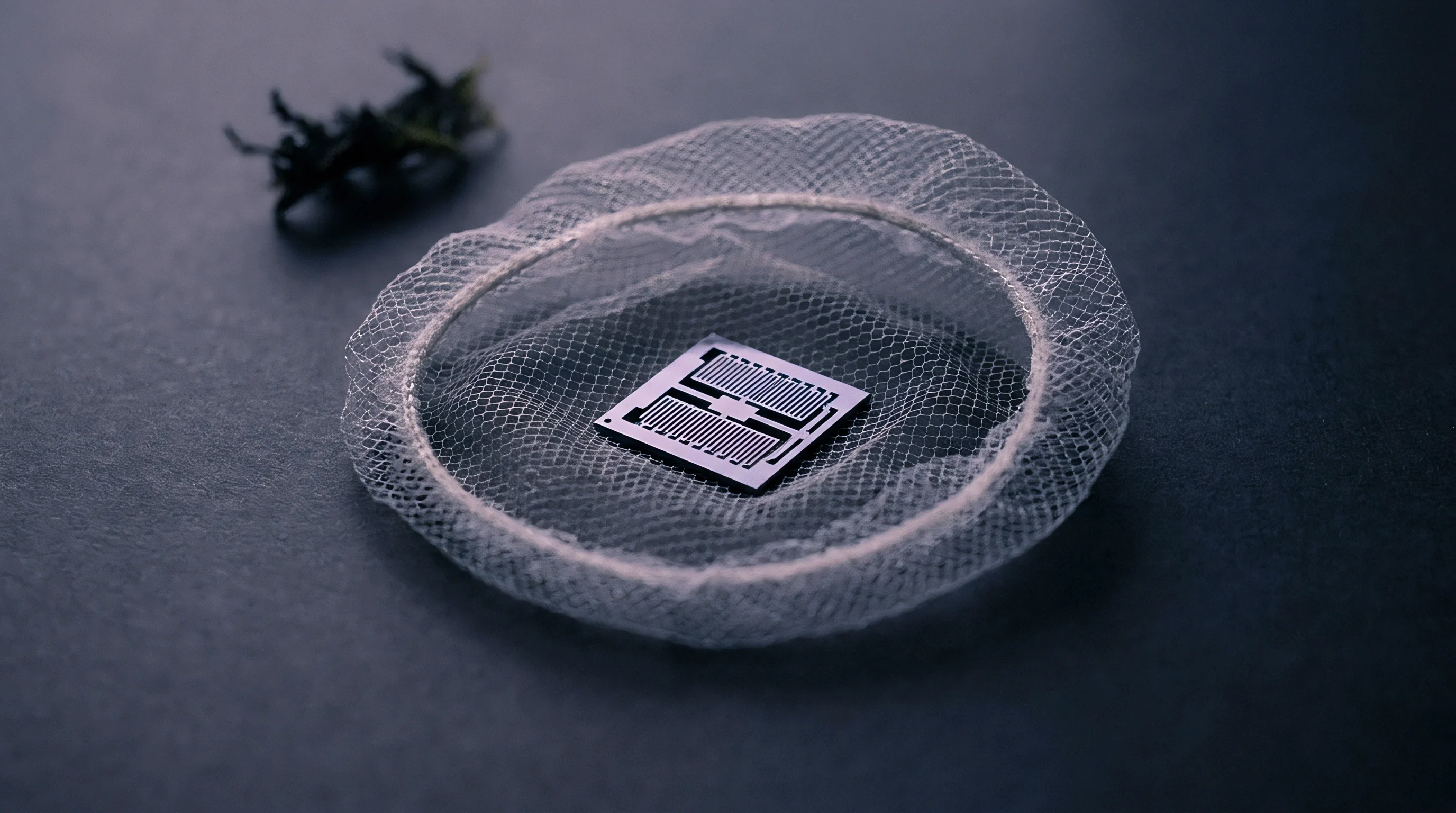
Mounting an inertial measurement unit onto an isolated granite surface within an environmental chamber isolates the silicon die from ambient building vibrations. The test fixture anchors to an active pneumatic damping table with resonant isolation below 1.5 Hz. Data acquisition boards pull continuous raw angular rate and specific force outputs over a serial peripheral interface bus at 1000 samples per second without hardware decimation filters enabled. Ambient chamber temperature stays regulated within a 0.1 °C boundary across forty-eight hours.
Decimation inside module firmware distorts the high-frequency slope. When an internal application-specific integrated circuit applies a cascaded integrator-comb filter or a finite impulse response rolling average, quantization noise collapses prematurely, masquerading as improved angle random walk. The bench operator bypasses digital smoothing blocks by polling raw register dumps directly from internal sensing channels.
Silicon dies respond to mounting torque. Mechanical clamping stresses induce thermal warping across solder joints, shifting apparent bias stability by 300 percent between bare boards and chassis enclosures.
IEEE 952 annex testing specifications govern drift validation by dictating rigid forty-eight hour environmental isolation windows during static calibration sweeps.
Data duration fixes parameter certainty. Extracting bias instability with ten percent confidence intervals dictates an observation period twenty times longer than the τ value at the curve minimum. When the curve flatlines at τ = 100 seconds, static acquisition continues uninterrupted for at least 2000 seconds.
Resolving rate random walk parameters at τ = 10,000 seconds dictates a stationary capture lasting beyond fifty hours.
Thermal Isolation and Logging Span
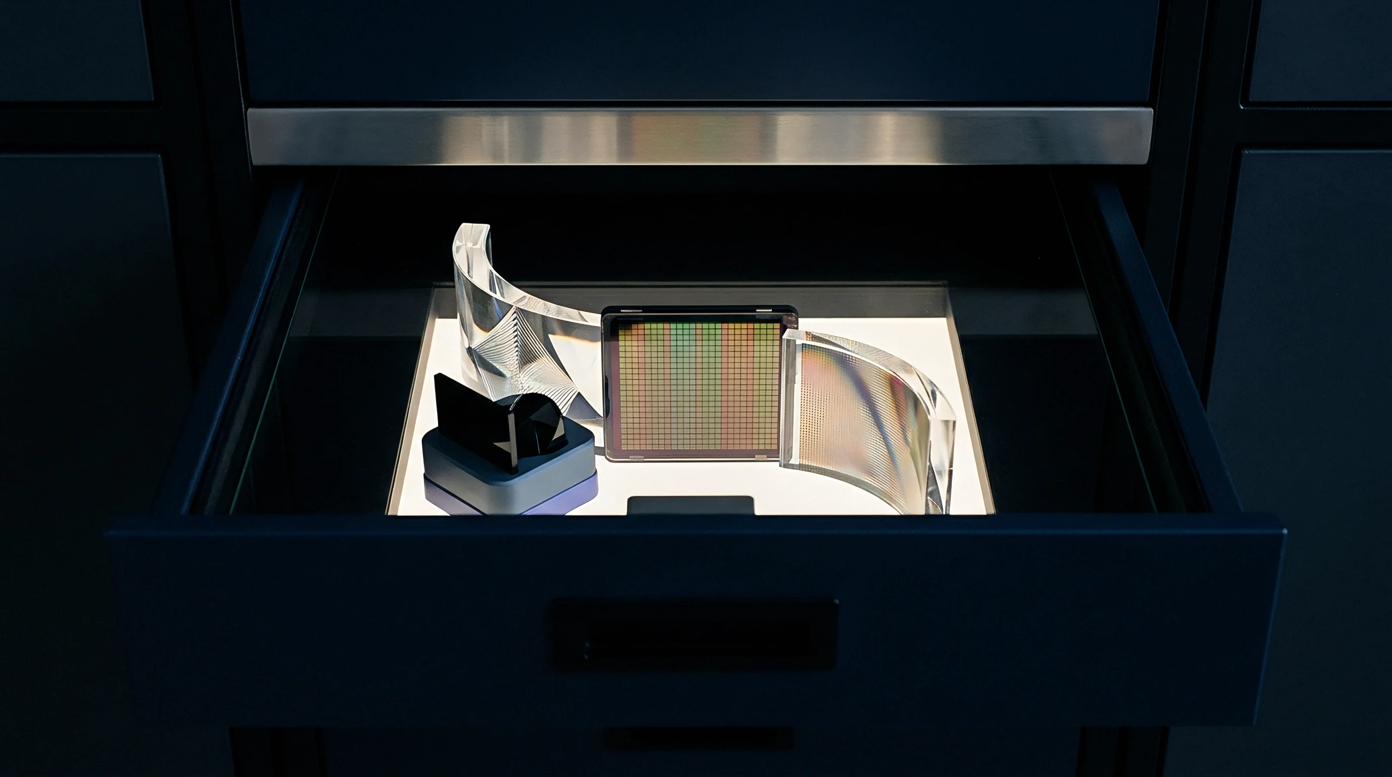
Chamber air currents introduce convective thermal gradients across ceramic ball grid array packages. Copper heat spreaders and foam baffles attenuate these gradients, preserving pure stochastic sensor behaviors. Thermal equilibrium dictates bias stability.
Logging raw sensor data during temperature cycling commingles deterministic temperature coefficients with true stochastic random walks, invalidating parameter extraction. Analysts separate deterministic bias temperature compensation tables from stochastic noise modeling by running Allan variance evaluations solely under isothermal conditions across multiple temperature setpoints.
| Performance Tier | Transduction Technology | Angle Random Walk (deg/√hr) | Bias Instability (deg/hr) | Rate Random Walk (deg/hr/√hr) | Logging Span (hr) |
|---|---|---|---|---|---|
| Consumer Mobile | Capacitive Surface MEMS | 0.300 to 0.900 | 12.0 to 35.0 | 1.50 to 5.00 | 12 |
| Industrial Automated | Tuning Fork MEMS | 0.060 to 0.150 | 2.0 to 6.0 | 0.20 to 0.80 | 24 |
| Tactical Avionics | Closed-Loop Silicon Resonator | 0.008 to 0.030 | 0.1 to 0.5 | 0.01 to 0.05 | 48 |
| Navigation Marine | Fiber Optic Gyroscope | 0.0005 to 0.002 | 0.002 to 0.01 | 0.0003 to 0.001 | 96 |
Verification protocols under IEEE standards enforce rigid environmental logging constraints, invalidating vendor datasheets that omit the duration, mechanical clamping torque, and chamber stabilization tolerance applied during characterization.
Conversion
Stochastic differential equations form the backbone of state estimation. For a continuous-time gyroscope error model, the true angular velocity vector relates to sensed velocity through an additive bias vector and zero-mean Gaussian white noise. The bias itself evolves as a random walk driven by an independent white noise vector.
Continuous-time spectral density matrices govern the dispersion rate of these stochastic inputs within the filter propagation loop.
The continuous process noise spectral density matrix Q_c incorporates the continuous white noise spectral density of the rate measurement q_rate and the continuous white noise spectral density driving the bias drift q_bias. These continuous densities derive directly from the extracted Allan variance parameters. The white noise spectral density q_rate equals the square of the angle random walk parameter N expressed in SI units: radians squared per second.
The bias random walk driving density q_bias equals the square of the rate random walk parameter K expressed in radians squared per second cubed.
A tactical-grade sensor characterized at 25 °C exhibits an angle random walk of 0.012 degrees per square-root hour, fixing continuous spectral density at 1.096e-9 radians squared per second.
Discrete Kalman filter algorithms execute at finite update intervals Δt. The continuous state propagation model converts to discrete process noise covariance Q_k through integration of the continuous spectral density projected through the system dynamics state transition matrix Φ(t). Numerical integration preserves the physical energy distribution across discrete steps.

Can Allan Variance Parameters Directly Populate Process Noise?
Raw parameters extracted from logarithmic plots cannot enter discrete covariance matrices without mathematical transformations involving the filter execution period Δt. Angle random walk represents an integrated white noise process, whereas rate random walk represents a second-order integrated process. Sample periods rescale discrete noise terms.
When an estimator runs attitude mechanization at 100 Hz (Δt = 0.01 s), the discrete angular covariance component scales proportionally with Δt, while bias dispersion components scale with higher powers of Δt.
Directly inserting static datasheet numbers into discrete covariance diagonals induces mathematical inconsistency. The filter designer evaluates the exact continuous-time differential equation before discretizing. For attitude error δθ and gyro bias error δb, the continuous state vector x = ^T evolves according to dx/dt = F x + G w, where F = and G =.
The noise vector w contains rate white noise w_rate and bias white noise w_bias with continuous covariance E = Q_c δ(t – τ).
Continuous Spectral Densities to Matrix Integrals
The discrete process noise covariance matrix Q_k evaluates through the matrix integral over the sample duration Δt: Q_k = ∫_0^Δt Φ(τ) G Q_c G^T Φ(τ)^T dτ. The state transition matrix Φ(τ) equals exp(F τ), which resolves for this system to. Multiplying the matrices inside the integrand and performing component-wise integration yields the complete discrete process noise covariance matrix.
The upper-left block of Q_k, governing attitude error covariance, equals (q_rate Δt + (1/3) q_bias Δt^3) I. The off-diagonal cross-correlation blocks between attitude error and bias error equal -(1/2) q_bias Δt^2 I. The lower-right block, governing bias error covariance, evaluates strictly to q_bias Δt I. Attenuation of the cross-coupling terms compromises filter stability when sample intervals widen. For high-rate systems where Δt is small, the (1/3) q_bias Δt^3 term vanishes relative to q_rate Δt, but the cross-coupling term preserves physical correlation between integrated angle drift and developing bias offsets.
| Identified Allan Parameter | Curve Gradient | Continuous Noise PSD (Q_c Element) | Discrete Covariance Formulation (Q_k / R_k) | SI Engineering Units |
|---|---|---|---|---|
| Angle Random Walk (N) | -1/2 | q_rate = N^2 | Q_θθ ≈ q_rate Δt | rad^2 / s |
| Rate Random Walk (K) | +1/2 | q_bias = K^2 | Q_bb = q_bias Δt | rad^2 / s^3 |
| Angle / Bias Cross-Coupling | Combined | Cross-term | Q_θb = -(1/2) q_bias Δt^2 | rad^2 / s^2 |
| Measurement White Noise | -1/2 | S_meas = N^2 | R_k = N^2 / Δt = σ_rate^2 | (rad / s)^2 |
| Bias Instability (B) | 0 | q_FOGM = 2 σ_BI^2 / τ_c | Q_FOGM = σ_BI^2 (1 – exp(-2 Δt / τ_c)) | (rad / s)^2 / s |
Failing to rescale spectral densities by the operating sample interval causes Kalman filter gains to diverge under variable loop execution rates, driving attitude estimates into unbounded oscillatory errors during dynamic maneuvers.

Discrepancy
Datasheet tables published by inertial sensor manufacturers regularly feature headline bias instability values stripped of practical context. Marketing summaries report the single absolute minimum point of a curated Allan deviation curve taken inside an oil-damped, magnetically shielded enclosure over sixteen hours. The reported figure represents the absolute optimum noise limit achievable by the transducer die under laboratory perfection.
In production hardware, bias instability behaves differently due to low-frequency package stress, board flexing, and linear acceleration rectification.
Flicker noise produces the flat bias instability region on an Allan deviation plot. Pure flicker noise possesses a power spectral density proportional to 1 / f, requiring an infinite number of states to model correctly in a linear state-space filter. Kalman filters accommodate finite state dimensions.
Designers approximate bias instability using a first-order Gauss-Markov process rather than a pure flicker model.
A simple mathematical convenience replaces infinite-order flicker noise with a bounded correlation interval.
The first-order Gauss-Markov approximation introduces a fictitious correlation time τ_c, chosen to match the duration of the flat minimum on the Allan deviation curve. The state equation becomes db/dt = -(1 / τ_c) b + w_GM, where the variance of the driving white noise w_GM evaluates to 2 σ_BI^2 / τ_c, with σ_BI representing the Allan variance bias instability floor. Selecting τ_c requires subjective judgment.
Engineering teams dispute whether τ_c belongs at 100 seconds, 500 seconds, or 1000 seconds.
Which Noise Terms Dominate Short Horizons?
Navigation systems running on brief duty cycles depend primarily on angle random walk rather than bias instability or rate random walk. For integration windows under ten seconds, angle random walk accounts for over ninety percent of orientation variance. The sample clock sets the horizon.
Bias instability only begins to dominate error budgets once integration intervals exceed the crossover time where σ(τ) flattens out.
Neglecting mathematical rigor during parameter conversion induces severe operational degradation across predictable phases:
- Underestimating measurement noise covariance causes the Kalman filter to over-trust individual sensor readings, injecting high-frequency digitizer noise into estimated state velocities.
- Omitting cross-coupling covariance components forces state projection gains to ignore correlation, creating artificial divergence between attitude angles and estimated sensor biases.
- Assigning arbitrary Gauss-Markov correlation times creates mismatched Kalman gains that either lag behind true physical drift or over-correct stable bias baselines.
- Ignoring thermal hysteresis shifts produces steady-state estimation offsets that external aiding measurements fail to reconcile without inflating process noise bounds.
Suppliers routinely dismiss bench deviations by asserting that factory qualification sweeps characterize die intrinsic performance rather than secondary board assembly degradation.
Exposure
Sourcing commercial MEMS inertial measurement units introduces supply chain risks tied directly to internal die architecture. Multi-axis sensors from distinct fabrication foundries share mechanical packages and pinouts while operating on divergent physical sensing principles. One manufacturer utilizes a single proof mass with capacitive comb-drive sensing in an evacuated cavity, whereas another utilizes separate multi-ring resonators vibrating under high vacuum with piezo-resistive readout bridges.
While both components quote 0.05 degrees per square-root hour on their front page, their long-term drift characteristics differ completely.
Swapping pin-compatible parts without retuning discrete process noise matrices in vehicle software degrades navigation guidance. A change in cavity gas damping shifts internal mechanical quality factors, altering white noise distribution across high frequencies. Quartz timing crystal packages and hermetic ceramic seals exhibit similar packaging mechanics, where trace moisture leakage degrades long-term frequency stability over years of storage.
If an alternate sensor exhibits an Allan variance minimum at τ = 30 seconds instead of the qualified vendor’s τ = 300 seconds, the operational filter operates with stale covariance matrices.
Procurement teams protect production schedules by demanding comprehensive Allan variance qualification dossiers within the initial request for quotation. The procurement specification defines mandatory bench recording constraints:
Static logging must span seventy-two consecutive hours at 25 °C within a thermally controlled chamber. The supplier delivers raw, un-decimated time-series data captured at the native internal analog-to-digital conversion rate alongside calculated Allan deviation plots. Sample batches include components from at least three distinct wafer lots to characterize run-to-run parameter dispersion.
Sourcing agreements require advance notification whenever modifications occur in foundry etching recipes, wafer capping pressures, or application-specific integrated circuit decimation registers.
Second-source qualification costs extend beyond basic component unit pricing. Auditing raw time-series data, regenerating Allan variance profiles, re-tuning discrete Kalman filter process covariance matrices, and re-validating state estimation performance across environmental chambers requires four to six weeks of engineering bench time per alternate component. Whether future multi-die silicon packaging standards will unify internal damping parameters and thermal drift dynamics across competing MEMS foundries remains an open commercial question.