Deep Ocean Conductivity Sensor Hydrostatic Pressure Calibration
Hydrostatic pressure distorts ocean conductivity cells, requiring high-pressure calibration to isolate physical cell compression from thermodynamic fluid changes.
Deformation
Volumetric Strain in Deep Ocean Cell Geometries
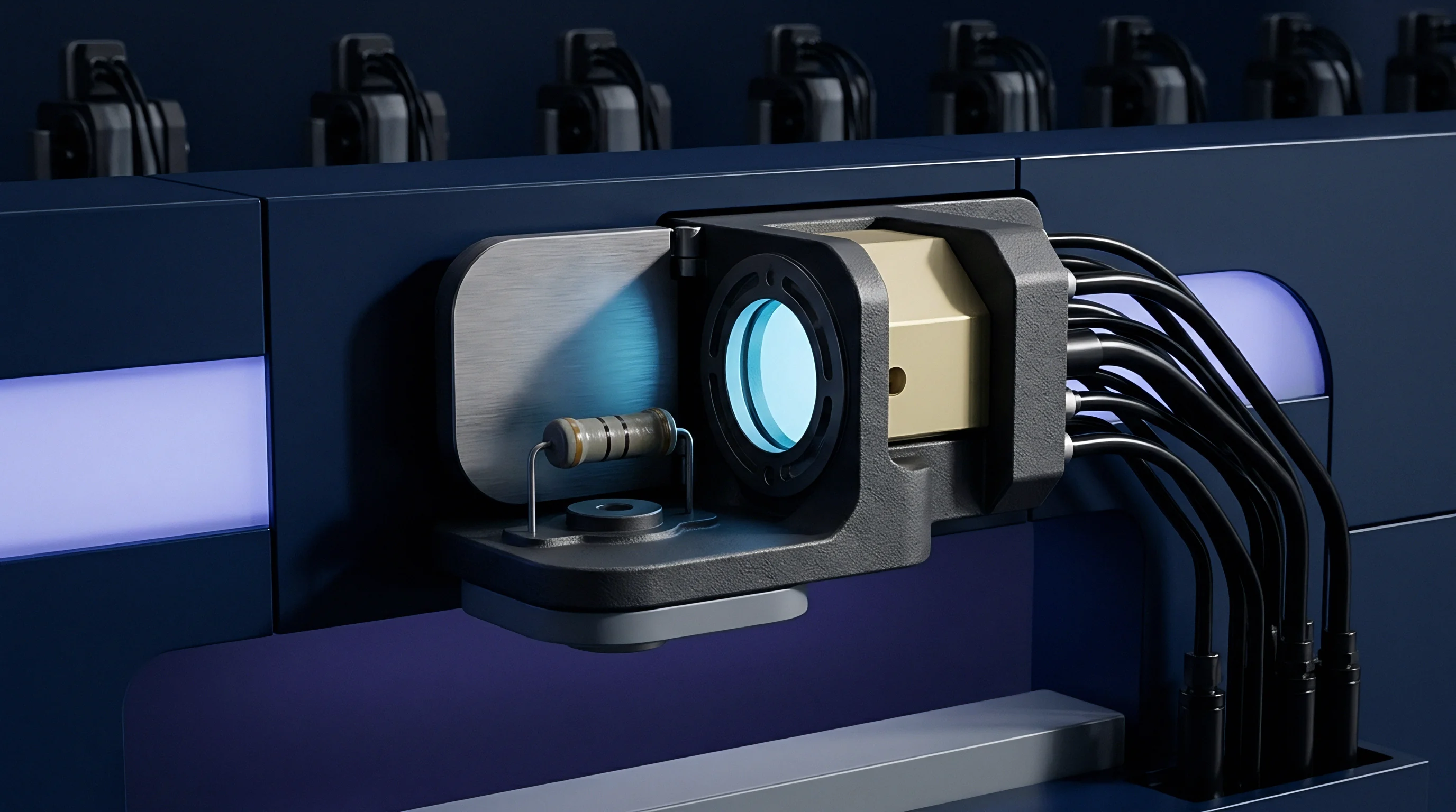
At hydrostatic pressures reaching 6000 decibars in deep ocean trenches, physical sensing elements undergo isotropic volumetric compression. The fundamental measurement of seawater electrical conductivity relies on determining the conductance of a fluid volume contained within a geometrically fixed path. This spatial path defines the cell constant, expressed as the ratio of effective length to cross-sectional area.
Hydrostatic pressure alters both dimensions simultaneously, shrinking the physical envelope of the sensing channel.
For electrode-based cells constructed from borosilicate glass, fused quartz, or ultra-pure alumina ceramics, uniform isotropic pressure reduces the internal bore diameter while shortening the axial distance between measuring electrodes. Because volumetric contraction reduces internal cross-sectional area faster than it shortens axial length, the geometric cell constant increases under compression. If uncorrected, this physical contraction causes the sensor to output a lower electrical conductance reading than the actual fluid conductivity dictates, introducing a salinity error that scales linearly with water depth.
Inductive Toroid versus Electrode Cell Mechanics
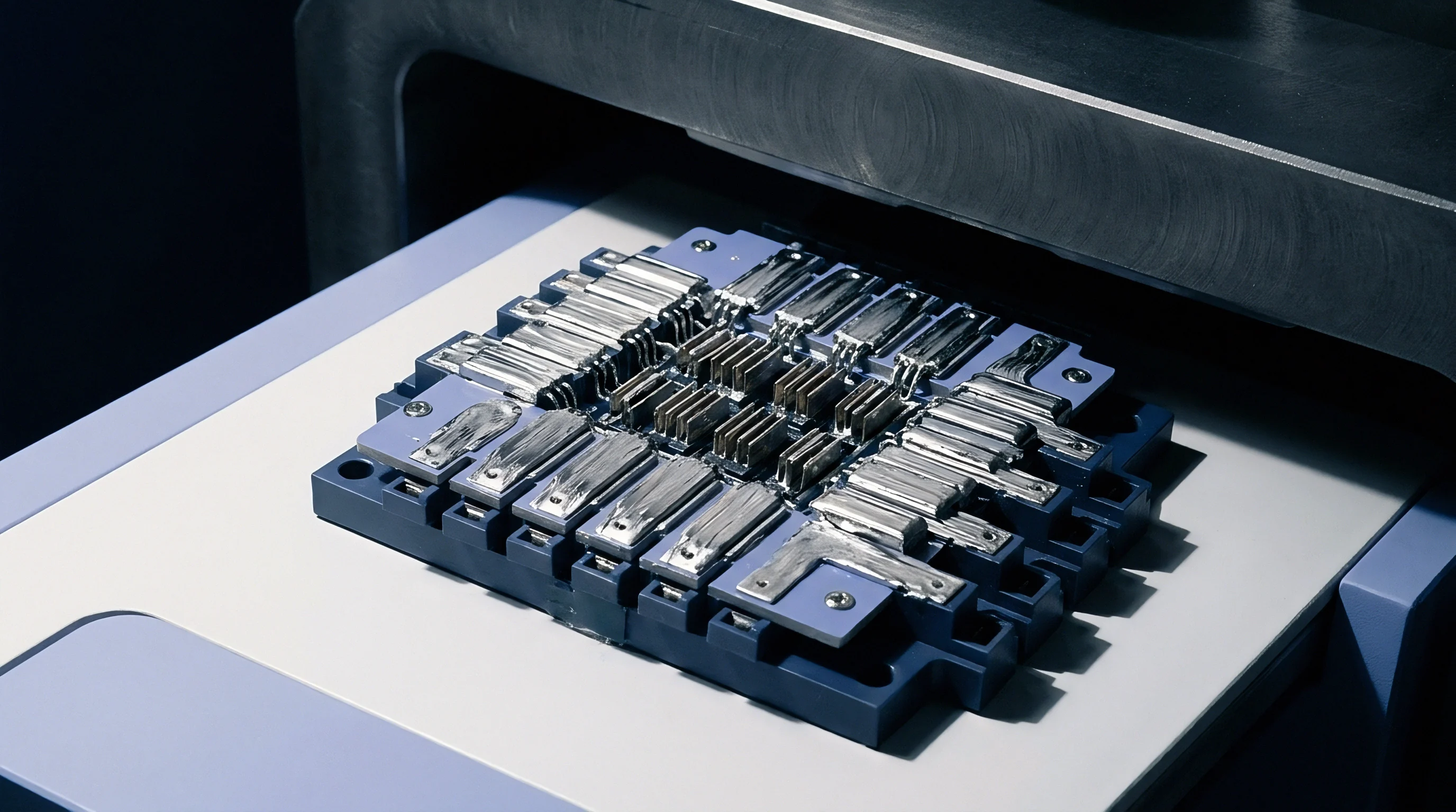
Inductive conductivity sensors rely on dual toroidal transformers encased in a protective outer housing rather than direct fluid-contact electrodes. Seawater passes through a central bore hole, forming a single-turn conductive loop that couples the primary excitation toroid to the secondary receiver toroid. The housing material surrounding these magnetic cores dictates the structural response under deep ocean hydrostatic loading.
Polymeric housings such as polyurethane or polyether ether ketone experience far higher compressible strain than ceramic or quartz channels.
Polymer housings compress under deep ocean loading, altering the internal diameter of the central bore and shifting the spatial geometry of the external current loop. Compression of the elastomeric material alters the effective path length of the seawater loop, generating a pressure-dependent scale factor shift. The physical compression mechanisms for common deep-sea sensing structures exhibit distinct mechanical signatures across depth ranges:
- Borosilicate Bore Compression reduces the cell cross-sectional area under pressure, elevating measured channel resistance and creating an artificial freshening offset in deep salinity calculations.
- Polyurethane Inductive Swell causes viscoelastic volume reduction around internal toroidal cores, shifting magnetic flux coupling under sustained hydrostatic pressure.
- Electrode Interface Displacement changes the physical gap between platinum voltage electrodes inside quartz channels, shifting the boundary layer calibration baseline.
- Alumina Ceramic Shrinkage maintains high structural stiffness up to 10000 decibars while undergoing small, linear, highly repeatable volumetric compression.
Failure to account for cell volume contraction under hydrostatic load distorts deep ocean water-mass identification. A false negative salinity drift of several thousandths of a Practical Salinity Unit obscures abyssal circulation patterns across ocean basins.
A borosilicate glass conductivity cell subjected to 6000 decibars of hydrostatic pressure undergoes volumetric compression that changes its cell constant by minus 0.00012 per thousand decibars at 2 degrees Celsius.
Thermodynamics

Decoupling Seawater Compression from Mechanical Contraction
Calculating seawater salinity relies on mathematical algorithms that treat fluid electrical conductivity as a multi-variable function of temperature, salinity, and pressure. Hydrostatic pressure increases the real electrical conductivity of seawater independently of any sensor distortion. Compression brings dissolved sodium and chloride ions into closer spatial proximity, increasing ionic concentration per unit volume while enhancing ionic mobility through reduced fluid viscosity.
The Practical Salinity Scale of 1978 and the International Thermodynamic Equation of Seawater 2010 establish precise thermodynamic equations for the pressure dependence of ocean water conductivity. Calibrating a deep ocean sensor requires separating the thermodynamic conductivity increase of the fluid from the mechanical cell compression factor. Laboratory testing inside high-pressure vessels isolates these two co-occurring phenomena by comparing raw sensor output against the theoretical thermodynamic response of standard seawater at identical temperature and pressure points.
Polynomial Corrections in Practical Salinity Calculations
Correcting raw sensor readings requires applying a hydrostatic compressibility correction factor, designated as beta, to the cell constant. The mathematical model modifies the atmospheric cell constant using a linear or second-order pressure polynomial. The corrected conductivity equals the raw measured conductivity divided by the product of one plus the thermal expansion correction and one minus the pressure correction term.
The mechanical compressibility coefficient beta varies across cell geometries and material compositions. Ceramic cells exhibit low beta values with minimal temperature dependence. Glass cells display moderate beta values that remain stable over thousands of pressure cycles.
Polyurethane-potted inductive sensors require second-order polynomial terms to capture non-linear compression across broad depth ranges.
| Cell Material | Nominal Beta (10^-6 / dbar) | Linear Thermal Expansion Alpha (10^-6 / K) | Hysteresis Index | Pressure Limit (dbar) |
|---|---|---|---|---|
| Borosilicate Glass | -1.25 | 3.30 | Low | 7000 |
| High-Purity Alumina | -0.78 | 6.50 | Negligible | 11000 |
| Fused Quartz | -0.95 | 0.55 | Negligible | 10000 |
| Polyurethane Toroid | -3.40 | 150.00 | Moderate | 6000 |
| PEEK Housing Toroid | -2.10 | 47.00 | Low | 6000 |
Determining beta requires empirical testing inside accredited calibration chambers. Standard purchase agreements for oceanographic research equipment mandate certifying the beta coefficient across the full rated depth spectrum before field deployment.
Thermal equilibrium inside a high-pressure vessel settles completely after each pressure ramp before recording baseline conductivity, as adiabatic compression raises water bath temperatures and distorts raw cell readings.

Chamber
High Pressure Calibration Facility Architecture
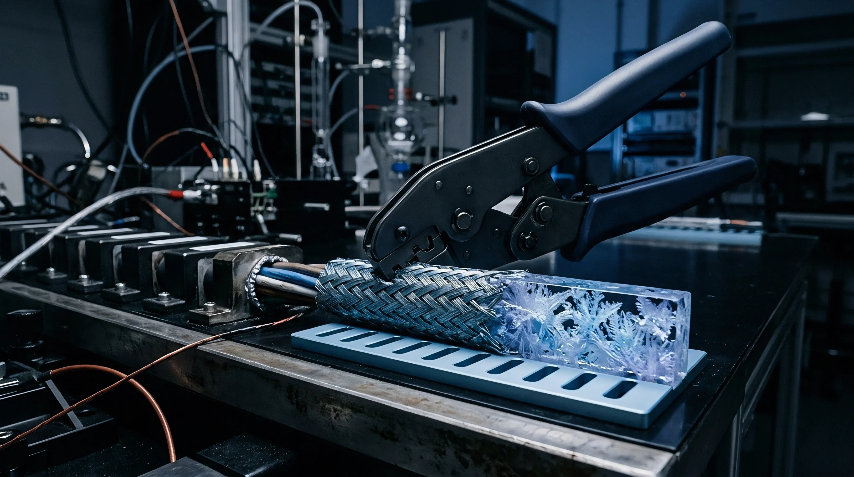
Simulating abyssal ocean environments requires pressure vessels engineered to withstand internal pressures exceeding 70 MPa while submerged in temperature-controlled liquid baths. Pressurizing fluid inside a closed vessel generates immediate adiabatic heating. Compressing standard seawater to 6000 decibars raises internal water temperature by approximately 1.5 to 2.0 degrees Celsius depending on initial starting temperature and pressurization speed.
High-precision calibration systems circulate fluid through high-capacity heat exchangers connected to external chiller baths to dissipate adiabatic heat. The temperature inside the calibration chamber must stabilize to within 0.001 degrees Celsius of the target setpoint before taking conductivity measurements. Primary pressure measurement relies on deadweight testers utilizing hydraulic piston gauges that provide primary pressure traceability.
These systems transfer pressure through automated oil-to-water isolators, keeping hydraulic oil out of the standard seawater circuit.
Step Pressure Profiling Procedure
Executing an accredited hydrostatic calibration involves stepping the sensor through a sequence of static pressure plateaus while monitoring temperature and cell conductance continuously.
- Submerge the oceanographic conductivity cell inside the high-pressure vessel filled with IAPSO standard seawater of certified practical salinity.
- Stabilize the surrounding liquid bath temperature at 2.000 degrees Celsius for four hours to eliminate internal vessel temperature gradients.
- Increase internal hydrostatic pressure in 1000-decibar increments up to the maximum operating rating of the sensor assembly.
- Hold system pressure static at each plateau for 45 minutes to permit complete dissipation of adiabatic heat and achieve thermal equilibrium.
- Record steady-state cell conductance once internal vessel temperature drift drops below 0.0002 degrees Celsius per minute.
- Depressurize the system in identical 1000-decibar steps to measure structural hysteresis and mechanical relaxation during unloading.
Ambient calibration combined with theoretical material compressibility figures is sometimes substituted for high-pressure testing, though uncalibrated polymer compression variations produce unacceptably high measurement errors during deep hydrographic surveys.
Budget

Uncertainty Component Identification under Pressure
Quantifying measurement certainty for deep sea conductivity sensors demands rigorous compilation of both statistical variations and systematic equipment errors. ISO/IEC Guide 98-3 standard uncertainty propagation protocols apply directly to high-pressure calibration data. Standard seawater salinity uncertainty forms the foundational baseline of the budget, where batch-to-batch variations in certified standard seawater introduce uncertainty into baseline fluid conductivity calculations.
Temperature bath instability inside the pressure vessel represents a dominant source of error. Because seawater conductivity changes by roughly two percent per degree Celsius, a thermal fluctuation of 0.001 degrees Celsius shifts measured conductivity by 0.001 mS/cm. Additional uncertainty contributions arise from piston gauge pressure reference tolerances, sensor electronic noise floors, and pressure hysteresis during depressurization cycles.
Combined Standard Uncertainty Calculation
Evaluating standard uncertainties requires calculating sensitivity coefficients that translate individual parameter errors into equivalent conductivity units. The combined standard uncertainty equals the positive square root of the sum of squared product terms combining standard uncertainties with their respective sensitivity coefficients.
| Uncertainty Source | Type | Standard Uncertainty u_i | Sensitivity Coefficient c_i | Uncertainty Contribution (mS/cm) |
|---|---|---|---|---|
| Standard Seawater Salinity | B | 0.0015 PSU | 0.98 mS/cm per PSU | 0.00147 |
| Vessel Bath Thermal Stability | A | 0.0008 deg C | 0.91 mS/cm per deg C | 0.00073 |
| Piston Gauge Pressure Standard | B | 0.25 dbar | 0.00004 mS/cm per dbar | 0.00001 |
| Cell Mechanical Hysteresis | A | 0.0006 mS/cm | 1.00 unitless | 0.00060 |
| Sensor Signal Electronics Noise | A | 0.0003 mS/cm | 1.00 unitless | 0.00030 |
| Combined Standard Uncertainty (k=1): 0.00178 mS/cm | Expanded Uncertainty (k=2, 95% Confidence): 0.00356 mS/cm | ||||
Lowering total uncertainty in deep calibration relies more on controlling bath thermal stability than on increasing the precision digit count of the pressure transducer.
Failure to include cell mechanical hysteresis in the overall uncertainty calculation invalidates compliance with marine observation standards for deep ocean monitoring below two thousand meters.
Wander

Viscoelastic Creep in Sensor Materials
Extended submergence at abyssal depths induces material relaxation in sensor assemblies that does not reverse immediately upon surfacing. Polymers used in inductive toroid encapsulation, potting resins, and O-ring seals undergo slow viscoelastic creep when subjected to continuous hydrostatic pressure for months or years. This creep alters the physical dimensions of the cell housing over time, causing continuous zero-point wander and span drift.
Glass and ceramic electrode cells experience virtually no viscoelastic creep within their bulk crystalline or amorphous structures. Micro-straining around titanium end-caps, potting interfaces, and glass-to-metal electrical feedthroughs introduces subtle structural shifts under sustained load. Field deployments on deep ocean moorings require distinguishing between rapid mechanical relaxation and gradual sensor drift caused by surface contamination or biofouling.
Long Term Mooring Drift under Sustained Deep Pressure
Quantifying calibration drift after long-term deep sea deployment demands structured verification procedures upon instrument recovery. The sensor housing must undergo immediate inspection and pre-cleaning calibration checks to capture the raw state of the instrument before mechanical handling disrupts settled components.
- Baseline Zero Check measures atmospheric signal offset in clean air immediately upon instrument recovery to verify electronic zero-point stability.
- Post-Recovery Bath Comparison evaluates returned sensors in temperature-controlled standard seawater to quantify raw calibration drift prior to cleaning.
- Dual-Ramp Pressure Testing executes consecutive ascending and descending pressure calibration cycles to isolate reversible elastic deformation from permanent material creep.
- Coefficient Adjustment Protocol updates the pressure correction factor beta independently from ambient temperature coefficients to preserve baseline factory calibrations.
The precise micro-structural mechanism that causes potted inductive toroid geometries to retain residual deformation after eighteen months at six thousand decibars remains open to empirical dispute among polymer metrologists.
A conductivity sensor calibrated only at atmospheric pressure can accumulate an error equivalent to three meters of water column depth equivalent in density calculations when deployed at the abyss.
Ledger
Calibration Tier Cost Structures
Procurement decisions for deep sea instrumentation balance initial capital outlay against the operational risk of uncalibrated measurement errors. Purchasing a sensor with a simple atmospheric pressure calibration certificate minimizes upfront procurement expenses, but deploying that sensor into abyssal oceanographic campaigns introduces systematic errors that compromise research integrity and data validity.
High-pressure metrology laboratories operate specialized autoclave systems, high-capacity temperature control baths, and primary piston gauges. Certification costs scale directly with the number of pressure and temperature calibration points required across the target operating matrix. Oceanographic programs allocate specific funding lines for initial multi-point pressure calibration and recurring post-recovery calibration checks.
Commercial Risk and Recalibration Intervals
Selecting an appropriate calibration tier depends on deployment depth, required measurement precision, and program duration. The financial risk of deploying unverified sensors includes potential data rejection by international ocean monitoring repositories, requiring costly repeat research cruises.
| Calibration Tier | Test Profile Parameters | Traceability Standard | Operational Cost (USD) | Deep Salinity Uncertainty (6000 dbar) |
|---|---|---|---|---|
| Tier 1 Standard Ambient | 1 Temp, 1 atm Pressure | NIST / PTB Ambient | 250 | 0.0150 PSU |
| Tier 2 Static Pressure | 3 Temps, 3 Pressure Steps | ISO/IEC 17025 Accredited | 1200 | 0.0050 PSU |
| Tier 3 Full Hydrostatic Matrix | 5 Temps, 7 Pressure Steps | Primary Piston Gauge / IAPSO | 3500 | 0.0015 PSU |
| Tier 4 Post-Deployment Verification | Full Matrix + Hysteresis Ramp | National Metrology Standard | 4800 | 0.0010 PSU |
The selection of calibration tier determines both initial landed cost and ongoing operational field budgets for oceanographic monitoring programs. Specifying full hydrostatic pressure matrix verification adds upfront testing expense, yet eliminates the far higher cost of invalidating multi-year deep sea research data sets due to uncalibrated cell compression errors.