Least Squares Bivariate Polynomial Surface Fitting for Piezoresistive Bridge Calibration
Bivariate polynomial surface fitting maps raw piezoresistive bridge ratios and temperatures to true pressure, suppressing thermal and non-linear drift below 0.05% FS.
Surface
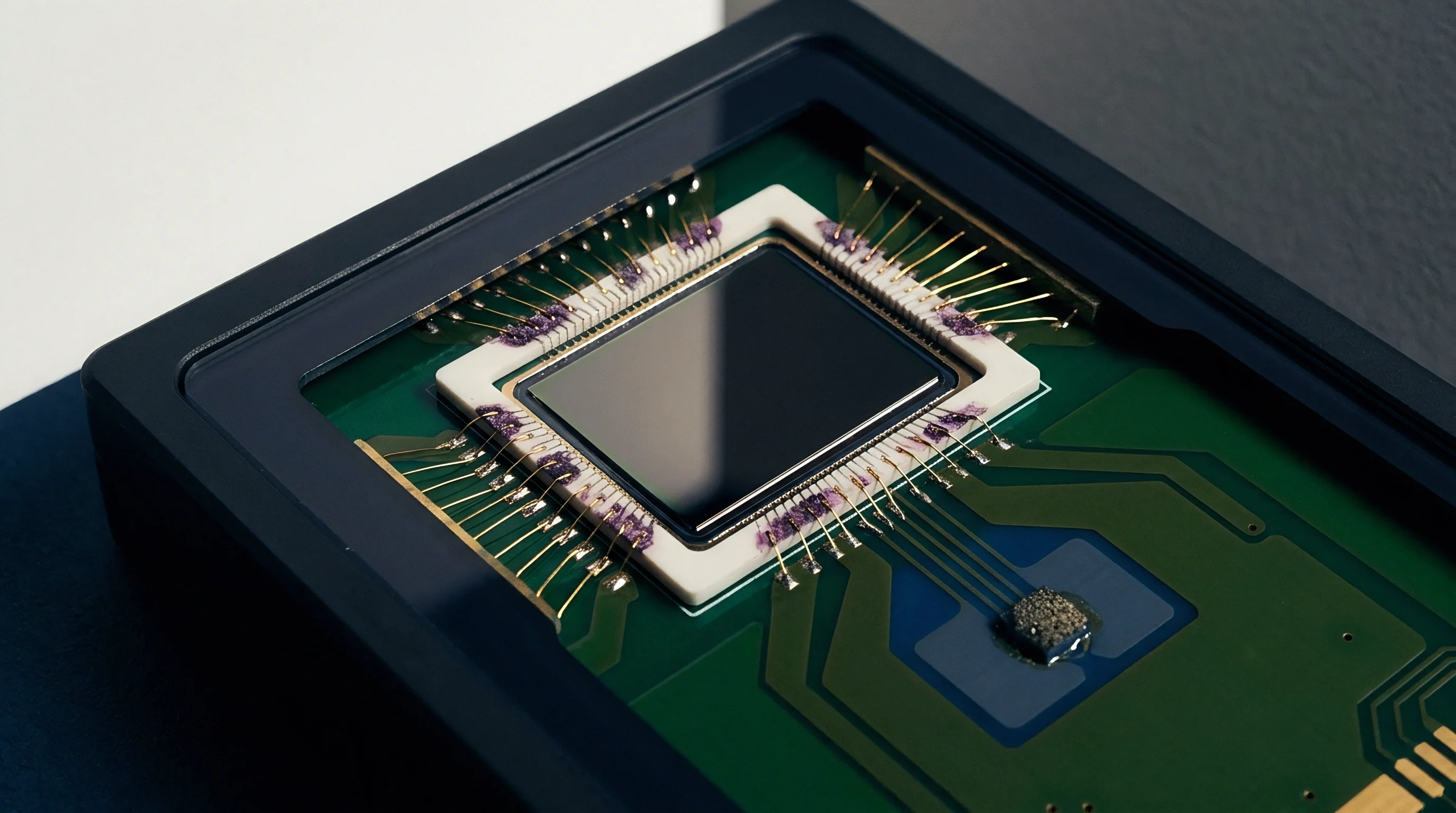
Piezoresistive silicon pressure sensors exhibit coupled non-linear responses across mechanical strain and ambient temperature. When pressure flexes an etched silicon diaphragm, embedded p-type resistors experience anisotropic stress that alters their electrical conductivity. Uncalibrated bridges exhibit wide thermal drift.
The differential voltage output shifts with mechanical load while simultaneously wandering due to the temperature coefficient of resistance and the temperature coefficient of piezoresistive sensitivity. These physical shifts prevent linear calibration models from achieving industrial accuracy targets across extended temperature ranges.
Bivariate polynomial mapping treats the sensor output as a continuous mathematical manifold spanning two physical dimensions. The transducer produces a raw bridge ratio, expressed as millivolts of differential output per volt of bridge excitation, alongside a temperature reading taken from an adjacent diode or bridge resistance monitor. Silicon piezoresistors exhibit negative sensitivity drift.
As temperature rises, carrier mobility in doped silicon decreases, causing the piezoresistive gauge factor to drop by roughly 1500 to 2200 parts per million per Kelvin. Mechanical stress concentrations across the perimeter of the diaphragm introduce geometric non-linearities at higher pressures. Bivariate fitting combines these independent variables into a single polynomial expansion that maps observed electrical states to calibrated engineering pressure units.
A piezoresistive bridge calibrated across minus forty to eighty-five degrees Celsius maintains an error band below 0.05 percent of full-scale span only when the mathematical model incorporates cross-axis terms.
Direct inversion models formulate true physical pressure as an explicit function of uncompensated bridge voltage and measured temperature. The mathematical representation expands as a double summation over specified polynomial degrees:
P(V, T) = sum from i=0 to M, sum from j=0 to N of a(i, j) multiplied by V to the power i, multiplied by T to the power j
In this formulation, V denotes the raw bridge output voltage ratio, T represents the measured temperature signal, a(i, j) designates the coefficient matrix, while M and N define the maximum polynomial degrees for voltage and temperature respectively. Cross terms capture mixed physical interactions. The coefficient a(1, 1) directly corrects the primary temperature coefficient of span, adjusting sensitivity as temperature alters the transconductance of the silicon piezoresistors.
Higher-order cross coefficients absorb secondary elastic distortions occurring when the silicon die expands at a different rate than its alumina carrier or glass constraint base.
Rig
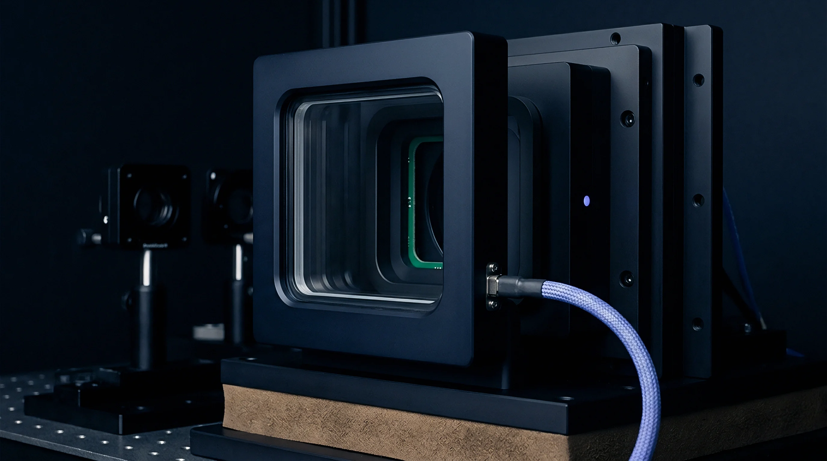
Extracting raw calibration points requires precise control of both mechanical pressure and thermal stabilization. Environmental chambers house automated pressure controllers alongside sensor fixtures to establish known physical setpoints across the operating envelope. Pressure manifolds house twelve sensors simultaneously.
Calibration fixtures incorporate high thermal mass copper blocks to minimize spatial temperature gradients across device housings during thermal soak cycles.
Pneumatic deadweight testers or digital quartz reference transducers generate pressure steps with reference uncertainties below 0.005 percent of reading. Thermal lag generates artificial hysteresis. If pressure data points are recorded before the sensor die reaches internal thermal equilibrium with the carrier header, the resulting polynomial absorbs dynamic transient lag rather than static physical characteristics.
Settling dwell times vary from fifteen minutes for miniature plastic packages to forty-five minutes for heavy stainless steel isolated diaphragms filled with silicone oil.
| Grid Configuration | Temperature Points | Pressure Points | Total Dwell Minutes | Mean Span Error Band |
|---|---|---|---|---|
| Sparse Orthogonal | 3 | 3 | 75 | 0.25 percent |
| Standard Industrial | 4 | 5 | 140 | 0.08 percent |
| High Precision Factorial | 5 | 7 | 225 | 0.03 percent |
| Overdetermined Extended | 6 | 9 | 360 | 0.02 percent |
Calibration chambers run automated scripts that cycle temperatures across the qualification limits before stepping pressure at each thermal plateau. Systematic bench errors alter raw calibration datasets when physical parameters drift unnoticed:
- Thermal gradient error develops when rapid air circulation inside the environmental oven cools fixture wiring faster than the package core, inducing parasitic Seebeck thermoelectric voltages across piezoresistor bond pads.
- Pressure head offset occurs when vertical displacement between the reference quartz barometer and the device under test shifts fluid head pressure by fractions of a millibar.
- Excitation source drift degrades voltage ratio calculations when bridge drive voltage wanders between baseline measurement cycles.
- Pneumatic manifold leakage introduces small continuous pressure drops that distort dwell plateaus during high-pressure data acquisition.
Contract manufacturing facilities often counter complaints about high calibration scatter by asserting that thermal equilibrium was achieved within fifteen minutes because chamber air thermometers had settled, despite the heavy stainless steel headers lagging behind.

Basis
Direct evaluation of raw polynomial terms introduces numerical degradation inside fitting algorithms. Raw bridge signals typically span dozens of millivolts, whereas temperature values expressed in Kelvin exceed several hundred units. Raising unnormalized integers to powers of three or four produces dynamic ranges exceeding twelve orders of magnitude.
Condition numbers exceed sixteen digits otherwise. Vandermonde design matrices populated with raw values exhibit extreme collinearity, which destroys numeric precision during floating-point matrix operations.
Normalization transforms raw hardware voltage and temperature counts into dimensionless values bounded between minus one and positive one before matrix decomposition.
Centering and scaling variables preserves numerical stability during execution. The calculation normalizes input variables through linear domain mapping:
u = 2 (V – V_min) / (V_max – V_min) – 1
v = 2 (T – T_min) / (T_max – T_min) – 1
The transformed coordinates u and v inhabit the closed interval between minus one and plus one. Substituting normalized values prevents higher-order powers from collapsing numerical rank during matrix inversion. Replacing standard monomial powers with orthogonal polynomial families improves stability across dense calibration grids.
| Polynomial Basis | Degree Formulation | Matrix Condition Number | Peak Residual Error |
|---|---|---|---|
| Raw Monomial | Biquadratic (2 by 2) | 4.2e+08 | 0.062 percent FS |
| Normalized Monomial | Biquadratic (2 by 2) | 1.8e+02 | 0.041 percent FS |
| Normalized Monomial | Bicubic (3 by 3) | 3.6e+04 | 0.018 percent FS |
| Chebyshev Bivariate | Bicubic (3 by 3) | 4.1e+01 | 0.016 percent FS |
Selecting appropriate basis functions balances mathematical expressiveness against edge oscillations:
- Monomial basis calculates powers directly from scaled inputs, maintaining minimal computation complexity during real-time microcontroller evaluation.
- Chebyshev basis utilizes recursive orthogonal trigonometric formulations that minimize maximum approximation error across the calibration domain.
- Legendre basis enforces mathematical orthogonality under uniform integration, preventing low-order coefficients from shifting when expanding model dimensions.
- Bicubic spline basis stitches localized third-order surfaces across partitioned sub-regions to eliminate non-linear ballooning anomalies without global polynomial divergence.
Higher degrees induce severe boundary oscillations. Adding excessive polynomial terms fits sensor noise rather than underlying transducer physics, degrading accuracy between calibration nodes.


Solver
Formulating the least squares problem constructs an overdetermined linear system X c = y, where X represents the design matrix containing evaluated basis terms, c denotes the unknown coefficient vector, and y contains true pressure reference values. Standard normal equations square condition numbers. Computing coefficients through the algebraic expression c = inverse(X_transpose X) X_transpose y doubles matrix condition numbers, provoking severe cancellation errors in finite-precision systems.
Householder reflections eliminate numerical inversion. Factorizing the design matrix via QR decomposition splits X into an orthogonal matrix Q and an upper triangular matrix R. The system reduces to R c = Q_transpose y, solved directly by backward substitution without squaring the underlying condition number. Singular value decomposition provides additional safeguards by decomposing X into unitary matrices U and V along with diagonal matrix S. Truncating near-zero singular values prevents noise magnification along weakly constrained polynomial dimensions.
Does Truncation Degrade Fixed Point ASIC Resolution?
Application-specific integrated circuits inside pressure transmitters execute surface evaluations using fixed-point arithmetic units to minimize die area and power consumption. Typical signal-conditioning chips dedicate sixteen to twenty-four bits of non-volatile memory to each polynomial coefficient. Converting double-precision floating-point coefficients into fixed-point representations introduces quantization steps that distort the calibrated surface.
- Construct the normalized design matrix X from observed chamber voltages and temperatures across all test nodes.
- Compute the QR decomposition of X to yield orthogonal matrix Q and upper triangular matrix R.
- Multiply the transpose of Q by the reference pressure vector to generate the transformed observation vector.
- Execute back substitution along upper triangular matrix R to extract the unconstrained floating-point coefficient vector.
- Quantize the resulting coefficients into target integer word lengths and simulate surface residuals across the dynamic range.
Fixed point rounding introduces quantization noise. Truncating low-order fractional bits shifts the zero-pressure baseline across temperature, producing uncorrectable systematic offsets in deployed field hardware.
Residual
Evaluating calibration quality requires analyzing difference surfaces generated by subtracting fitted values from known physical setpoints. Residual plots isolate physical sensor defects. A sound mathematical fit produces normally distributed residuals lacking spatial structure across the pressure-temperature domain.
Defects in sensor construction leave clear geometric signatures within residual distributions. An S-shaped residual curve along the pressure axis indicates unmodeled fifth-order mechanical ballooning in thin silicon diaphragms. A parabolic arch across the temperature axis reveals uncorrected second-order shifts in piezoresistor TCR.
Asymmetric spatial skewing highlights mechanical packaging stress transferred to the die through hardening room-temperature vulcanizing adhesives.
A surface model that leaves systematic ripples across the measurement domain indicates unmodeled packaging mechanics rather than mathematical fitting deficiencies.
Die attach adhesive relaxes under load. When packaging materials creep under high pressure, mechanical hysteresis offsets the return path, generating dual-valued readings that static bivariate polynomials cannot correct. Distinguishing mathematical under-fitting from transducer hysteresis prevents wasted engineering effort on polynomial expansion.
| Error Component | Raw Uncompensated Bridge | Analog Resistor Network | Bivariate Digital Fit | |
|---|---|---|---|---|
| Zero Thermal Drift | 12.5 percent FS | 1.20 percent FS | 0.02 percent FS | |
| Span Thermal Drift | -18.0 percent FS | 1.50 percent FS | 0.03 percent FS | |
| Pressure Non-linearity | 0.85 percent FS | 0.85 percent FS | 0.01 percent FS | |
| Mechanical Hysteresis | 0.02 percent FS | 0.02 percent FS | 0.02 percent FS | |
| Overall Accuracy Band | 31.37 percent FS | 3.57 percent FS | 0.08 percent FS | |
| Values represent typical limits across minus forty to one hundred twenty-five degrees Celsius. | ||||
Standard testing specifications defined in IEC 61298-2 mandate that non-conformity calculations account for dead-band errors and cyclic repeatability across consecutive thermal cycles, disallowing suppliers from masking mechanical hysteresis under mathematically averaged polynomial fits.

Ledger
Industrial deployment of surface calibration forces trade-offs between manufacturing throughput and final device yield. Environmental chamber cycle time represents the primary cost driver during automated sensor calibration. Holding twenty devices under test across five temperature plateaus consumes four hours of chamber time, tying up expensive pneumatic controllers and climatic ovens.
Sourcing fully calibrated digital pressure transmitters eliminates internal test infrastructure outlays while transferring margin to module packagers. Procuring raw uncalibrated silicon dies mounted to basic headers reduces component unit bills of materials by roughly sixty percent, yet demands capital investment in multi-manifold calibration chambers, deadweight calibrators, and custom automated test programming. High-volume manufacturing plants establish multi-site parallel testing manifolds to divide chamber overhead costs across hundreds of sensors per batch.
Purchasing raw piezoresistive bridge elements reduces upfront component expenditure but shifts calibration capital costs onto the production line.
Yield losses occur when individual dies exhibit thermal drift anomalies exceeding the compensation capacity of chosen polynomial models. If silicon dopant concentrations fluctuate across a single wafer run, piezoresistors produce erratic TCR curves that fail to conform to standard biquadratic surfaces. Manufacturers reject these out-of-family parts during calibration data processing, writing off both the silicon die and the chamber time spent acquiring data.
Whether fabless sensor manufacturers can reliably maintain low unit costs by training artificial neural networks on small batches to infer full surface coefficients from rapid two-point test cycles remains unresolved across modern automated production facilities.