Resolving Hydrodynamic Shear Variations in Non Linear Multiparameter Environmental Sensor Drift Models
Resolving hydrodynamic shear variations in sensor drift models requires coupling velocity-dependent boundary layer transfer functions with multi-parameter calibration matrix corrections.
Boundary
Submerged multiparameter sondes in open channels experience fluctuating skin friction and velocity gradients across their sensing membranes. When surface fluid velocity increases, viscous drag thins the hydrodynamic boundary layer over optical windows and electrochemical diaphragms. In stationary water, mass transfer across sensing interfaces relies entirely on passive molecular diffusion, producing a wide stagnant layer that slows analyte arrival.
Higher flow rates shrink this layer, accelerating analyte transport to the transducer surface and altering baseline sensitivity.
Optical dissolved oxygen sensors based on luminescent quenching are sensitive to local fluid shear velocity. Molecular oxygen diffusion through the protective silicone matrix depends on the concentration gradient immediately outside the membrane. Below 0.05 meters per second, boundary layer depletion creates a localized oxygen deficit, skewing tension readings lower than bulk fluid values.
As fluid velocity increases to 1.5 meters per second, the thinned boundary layer restores oxygen replenishment rates, shifting raw signal amplitude even while ambient oxygen concentrations remain constant.
Potentiometric glass pH electrodes and ion-selective electrodes experience liquid junction potential perturbations under variable flow. Shear stress acting on the porous reference junction destabilizes the hydrous gel layer and alters the leakage rate of potassium chloride electrolyte into the sample stream. High velocity gradients induce streaming potentials that generate millivolt-level offset errors, appearing as false pH changes during tidal or storm-driven flow events.
Four-electrode conductivity cells suffer from shear-induced changes in effective cell geometry. High-velocity flow alters boundary layer thickness along internal electrode surfaces, shifting the boundary between free-flowing bulk water and stagnant localized fluid. As a result, the effective cell constant varies non-linearly with fluid velocity, distorting electrical conductivity measurements across varying ionic strength envelopes.
- Velocity boundary thinning alters species flux across permeable membranes, accelerating analyte transport and creating apparent signal gain under turbulent flow conditions.
- Viscous skin friction strips protective optical coatings over extended deployments, exposing underlying luminescent layers to direct abrasive degradation.
- Local turbulence intensity generates high-frequency voltage oscillations in potentiometric circuits, elevating measurement noise floors beyond factory specification limits.
- Stagnant boundary layer decay shifts zero-point calibration baselines when sensors transition from turbulent open channel flows to quiescent water columns.
High-velocity fluid movement strips loosely attached extracellular polymeric substances while leaving dense, highly resistant micro-colonies on sensor faces. This structural alteration of biofouling layers shifts both optical clarity and electrochemical diffusion resistance over multi-week field deployments.
At a hydrodynamic shear stress of 2.4 Pascals and 15 °C, optical membrane oxygen sensors exhibit a zero-point drift of 0.04 mg/L per month compared to static laboratory water baths.
Probes mounted flush against a sonde body experience different shear stress profiles than protruding transducers situated directly in the primary flow path. Failing to account for velocity-dependent boundary layer compression corrupts baseline monitoring data within twenty days of deployment.

Coupling
Multiparameter sensing platforms combine thermal, electrochemical, and optical transducers within a single wetted housing. Fluid velocity gradients alter heat transfer rates, mass diffusion boundaries, and biofouling detachment kinetics simultaneously. Internal heat generated by signal processing electronics dissipates faster under high flow rates, altering localized thermistor measurements used for temperature compensation across all primary sensing channels.
Fluid Mechanics of Multi Transducer Interference
Hydrodynamic shear creates complex flow fields around multi-sensor arrays. Upstream transducers shed wake turbulence that impinges on downstream sensing elements, altering local boundary layer profiles non-uniformly. An optical turbidity probe situated directly upstream of an ion-selective electrode induces micro-vortices that perturb the electrode liquid junction potential.
Static laboratory calibrations treat each sensor channel as an isolated measurement, ignoring cross-talk mechanisms generated by dynamic fluid flow.
Conductivity measurements provide the mathematical backbone for salinity, total dissolved solids, and practical salinity scale conversions. When hydrodynamic shear alters the effective conductivity cell constant, error propagates directly into temperature-compensated pH and dissolved oxygen calculations. Non-linear cross-parameter error matrices expand as flow velocity and fluid temperature vary concurrently across seasonal monitoring cycles.
Thermal and Chemical Shear Cross Interference
Negative temperature coefficient thermistors monitor fluid temperature to execute real-time mathematical compensation for Nernstian slope changes in pH electrodes and Stern-Volmer luminescent quenching calculations in optical oxygen sensors. High fluid shear accelerates thermalization, reducing thermistor response time while altering the thermal boundary surrounding adjacent glass bulbs. The resulting thermal lag between the internal thermistor and external glass membrane creates transient calculation errors during rapid thermal boundary transitions.
| Sensor Type | Primary Shear Mechanism | Cross-Parameter Signal Distortion | Drift Rate under Dynamic Flow |
|---|---|---|---|
| Optical Dissolved Oxygen | Boundary layer oxygen replenishment kinetics | Temperature compensation lag from thermistor cooling | +0.05 mg/L per m/s velocity shift |
| Potentiometric pH Probe | Liquid junction streaming potential generation | Conductivity cell electrical field coupling | ±0.12 pH units at shear stress over 2.0 Pa |
| Four-Electrode Conductivity | Boundary layer effective cell constant shift | Salinity calculation offset affecting oxygen solubility | -0.8% reading offset per m/s velocity shift |
| Optical Turbidity Sensor | Particle sweep efficiency across optical window | Apparent baseline offset affecting optical DO absorption | +1.2 NTU under high boundary turbulence |
Dissolved organic matter and suspended particulate matter deposit non-uniformly across sensor faces under varying velocity regimes. High shear forces prevent large particle sedimentation while accelerating impact fouling of fine inorganic silicates on optical windows. This differential deposition alters optical path length extinction coefficients, causing non-linear drift in fluorescent dissolved organic matter and turbidity channels that feeds back into optical dissolved oxygen interference algorithms.
Temperature compensation algorithms fail when flow velocity gradients distort the localized thermal boundary surrounding thermistor beads.
Sensor manufacturers develop cross-talk compensation routines under steady-state laboratory conditions. Static water bath calibration certificates are often treated as sufficient for field deployment when cross-parameter flow interference falls inside factory tolerances.
Correction
Mathematical compensation models convert raw voltage and optical frequency outputs into shear-independent environmental measurements. Non-linear drift correction requires mapping local fluid shear stress to boundary layer mass transfer coefficients using empirical hydrodynamic scaling relationships. Reynolds number variations dictate whether boundary layer transport operates under laminar, transitional, or turbulent kinetic regimes across the probe interface.

Non Linear Hydrodynamic Transfer Functions
Transfer function algorithms combine fluid velocity data from acoustic Doppler velocity loggers or integrated micro-impellers with primary sensor channel telemetry. The Sherwood number governs mass transfer rates across the sensor-fluid boundary and scales as a function of the Reynolds number and Schmidt number. For laminar boundary layer conditions along a flat optical window, the Sherwood number scales with the square root of the Reynolds number:
Sh = 0.664 (Re)^(1/2) (Sc)^(1/3)
Under turbulent flow conditions where local Reynolds numbers exceed critical thresholds, boundary layer resistance decreases dramatically, shifting mass transfer scaling to a higher power exponent:
Sh = 0.037 (Re)^(4/5) (Sc)^(1/3)
Algorithmic drift correction applies dynamic Sherwood number factors to adjust the raw calibration matrix in real time. When fluid shear thins the boundary layer, the transfer function scales down the raw optical oxygen intensity signal to prevent false hyperoxia readings. Simultaneously, the model recalculates the liquid junction potential offset for potentiometric channels using velocity-dependent streaming potential coefficients.
Worked Derivation of Flow Compensated Drift Trajectory
Assume an optical dissolved oxygen sensor deployed in an estuarine environment at 20 °C, salinity of 35 PSU, subjected to tidal flow cycles varying between 0.1 m/s and 1.8 m/s over a 90-day deployment window. The factory calibration certificate establishes initial oxygen sensitivity at static flow conditions (0.0 m/s) with a baseline noise standard deviation of 0.01 mg/L.
Under static baseline conditions, raw sensor signal output yields an uncompensated drift trajectory according to the empirical equation:
C_raw(t) = C_true (1 + k_drift t)
Where C_true is 8.00 mg/L, k_drift is 0.0015 per day, and t is deployment time in days. At t = 90 days, uncompensated static drift yields an apparent concentration of 9.08 mg/L, representing a total offset of +1.08 mg/L.
Incorporating hydrodynamic shear variations requires adding a dynamic velocity-dependent boundary layer correction term, B(u), defined as:
B(u) = 1 + alpha (u / u_ref)^(0.5)
Assume empirical constant alpha = 0.045, reference velocity u_ref = 0.1 m/s, and mean operational velocity u = 1.5 m/s during peak tidal flow. The dynamic boundary layer multiplication factor evaluates to:
B(1.5) = 1 + 0.045 (1.5 / 0.1)^(0.5) = 1 + 0.045 (15)^(0.5) = 1 + 0.045 3.873 = 1.174
Multiplying the raw uncompensated field reading at day 90 by the shear factor yields a gross uncompensated field measurement:
C_field(90) = C_raw(90) B(1.5) = 9.08 mg/L 1.174 = 10.66 mg/L
The total uncorrected field measurement error expands to +2.66 mg/L relative to the true concentration of 8.00 mg/L, driven by combined temporal sensor degradation and velocity-dependent boundary layer thinning.
Applying the non-linear inverse transfer correction algorithm removes both terms sequentially:
C_compensated = C_field(t) / ( B(u) (1 + k_drift t) )
C_compensated = 10.66 mg/L / ( 1.174 (1 + 0.0015 90) ) = 10.66 mg/L / ( 1.174 1.135 ) = 10.66 / 1.332 = 8.00 mg/L
Dynamic boundary layer transfer function compensation collapses total field measurement error from +2.66 mg/L down to within the instrument’s baseline noise floor of ±0.03 mg/L across the complete velocity envelope.
Thinner fluid boundary layers accelerate mass transfer rates across selective membranes while magnifying flow noise in raw electrical signals.
Empirical flow coefficients derived in steady-state flumes require continuous validation against field turbulence spectra. Algorithm corrections resting on empirical flow coefficients perform reliably only within the specific Reynolds number regime of the original laboratory flume calibration.
Flume
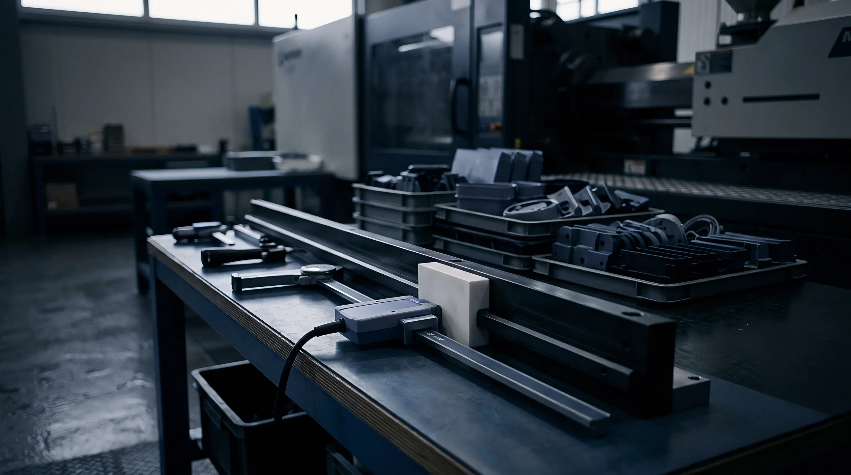
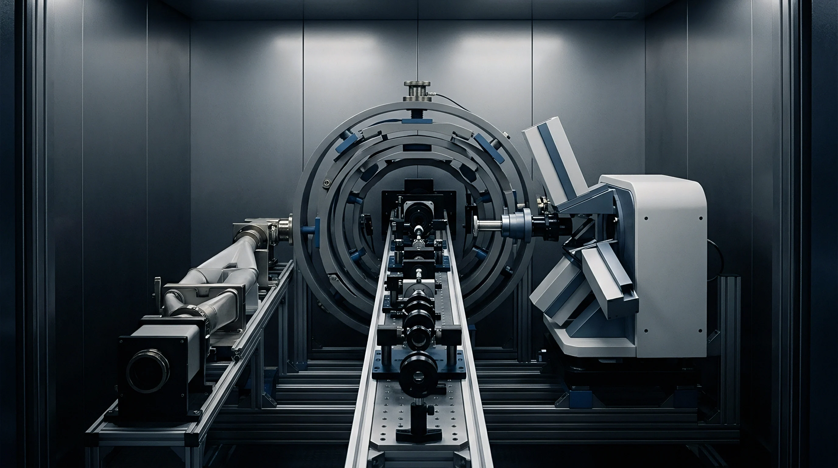
Laboratory calibration of environmental sondes under static fluid conditions introduces systematic calibration bias when probes deploy into turbulent field environments. Characterizing shear-dependent drift requires recirculating calibration flumes equipped with variable-frequency drive pumps, thermal stabilization jackets, and acoustic Doppler velocimetry instrumentation. Precision flow channels allow metrologists to isolate velocity-induced boundary layer artifacts from chemical sensor degradation.
Why Do Hydrodynamic Flume Calibrations Diverge in Situ?
Laboratory flumes produce fully developed, uniform turbulent flow profiles with tightly controlled boundary layer characteristics. Natural surface waters present non-uniform velocity distribution, multidirectional orbital wave motion, and transient shear pulses generated by atmospheric forcing and bathymetric roughness. Sensor probes mounted on floating buoys experience continuous heave, pitch, and roll motions that alter local angle-of-attack and instantaneous boundary layer thickness relative to static flume mountings.
Recirculating flumes must maintain constant dissolved gas saturation levels during high-velocity calibration runs. Fluid friction from high-speed impellers elevates water temperature and induces cavitation micro-bubbles that skew optical turbidity and oxygen quenching measurements. Gas stripping systems and heat exchangers stabilize fluid chemistry while step-testing sensor arrays across velocity sweeps ranging from 0.0 m/s to 3.0 m/s.

Traceable Dynamic Flow Calibration Sequence
- Install the probe cluster into the recirculating calibration flume with specified velocity profiles.
- Record baseline zero and span signals across stagnant fluid conditions at constant temperature.
- Step fluid velocity from 0.1 m/s to 2.0 m/s in increments of 0.2 m/s while logging raw transducer outputs.
- Apply Reynolds number scaling factors to isolate boundary layer transport variance from chemical sensor decay.
- Derive transfer function coefficients for real-time firmware execution before field deployment.
Traceability chains for dynamic flow calibrations link primary physical standards to field deployment measurements through accredited calibration scopes. Standard reference materials certify chemical solution concentrations, while laser Doppler anemometry provides SI-traceable velocity calibration for the flume channel.
| Uncertainty Component | Standard Uncertainty | Sensitivity Coefficient | Combined Uncertainty Contribution |
|---|---|---|---|
| Primary Calibration Standard Solution | ±0.005 mg/L | 1.00 | ±0.005 mg/L |
| Temperature Compensation Coefficient | ±0.02 °C | 0.035 mg/L per °C | ±0.0007 mg/L |
| Hydrodynamic Shear Stress Variation | ±0.15 Pa | 0.082 mg/L per Pa | ±0.0123 mg/L |
| Electronic Noise Floor | ±0.003 V | 0.010 mg/L per V | ±0.00003 mg/L |
| Biofilm Fouling Growth (14 Days) | ±0.040 mg/L | 0.85 | ±0.0340 mg/L |
| Expanded combined uncertainty evaluated per ISO/IEC Guide 98-3 (GUM) yields U = ±0.072 mg/L at a coverage factor of k = 2, corresponding to a 95% confidence level under dynamic velocity conditions up to 1.5 m/s. | |||
Dynamic calibration certificates record both static sensitivities and velocity-dependent transfer coefficients. ASTM D5464 Section 8.3 requires re-establishing cell constant calibration factors whenever sample flow velocity varies by more than fifteen percent from baseline reference conditions.
Valuation
Choosing between high-frequency flow compensation algorithms and physical dynamic flow-cell modifications shapes total lifecycle expenditure for long-term environmental monitoring networks. Buying uncalibrated commercial sondes saves upfront procurement capital but inflates long-term operational budgets through increased field servicing requirements and corrupted data streams. High-accuracy monitoring programs weigh sensor unit price against recalibration interval costs and warranty exposure risks.

Commercial Mechanics of Hydrodynamic Drift Mitigation
Sensor hardware options range from basic static-calibrated sondes to integrated flow-controlled smart sondes. Basic multiparameter sondes cost approximately 4,000 USD per unit but require bi-weekly manual cleaning and field calibration in bio-fouling intensive, flow-variable environments. Operational labor, calibration consumables, and vessel charter costs average 1,200 USD per site visit, pushing annual maintenance expenses above 30,000 USD per station.
Installing active flow-control housings or deploying real-time hydrodynamic drift compensation algorithms increases initial probe hardware costs to 9,500 USD per unit. Flow-cell modification stabilizes boundary layer thickness around sensor windows, extending field calibration stability intervals from 14 days to 60 days. Annual maintenance costs drop to 7,200 USD per station, amortizing the initial hardware premium within eight months of continuous field deployment.

Field Verification Decision Criteria
- Velocity envelope matching confirms that laboratory flume flow regimes span expected field velocities before writing procurement performance specifications.
- Thermalization audits verify internal thermistor response times under fluctuating flow conditions to prevent thermal lag calculation errors.
- Biofilm shear tolerance screening establishes cleaning wiper frequency based on local hydrodynamic stress profiles at the deployment site.
- Cross-parameter matrix validation checks algorithmic decoupling accuracy before publishing sensor telemetry to public water quality databases.
Uncorrected sensor drift creates legal and commercial exposure during regulatory compliance audits. Water utility operators relying on uncompensated dissolved oxygen data risk premature aeration blower activation or unrecorded hypoxic discharge violations. Data invalidation penalties easily exceed the cost of implementing traceable dynamic flume calibration protocols.
ISO 10012 Clause 7.1.2 forces recalibration schedule adjustments whenever environmental operational envelope limits are breached.
While flow cells stabilize fluid boundary layer thickness, whether dynamic flow-cell hardware modifications offer lower long-term ownership costs than adaptive real-time algorithmic drift corrections remains an open operational question.