Quantifying Thermal Soak Delays in Encapsulated Process Temperature Sensors
Quantifying thermal soak delays requires isolating sheath resistance and fill conductivity to offset dynamic tracking errors in automated process control loops.
Sheath
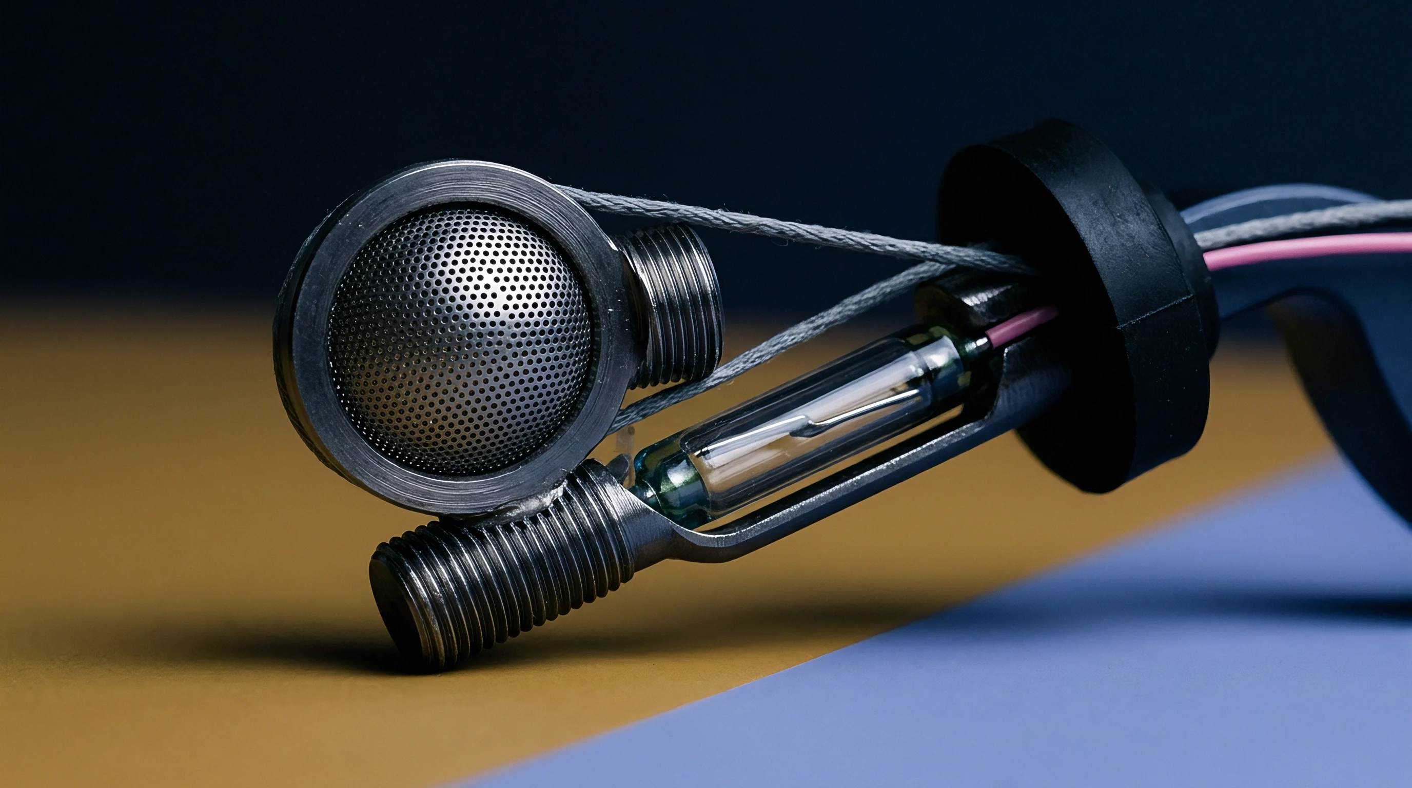
Process temperature sensors installed in industrial thermowells rely on potting compounds and metal sheaths to isolate delicate platinum resistance elements from high pressure, mechanical vibration, and corrosive process fluids. That protective barrier, however, creates an unavoidable series of thermal resistances. Whenever the pipe temperature shifts, heat must cross the external fluid boundary layer, the thermowell wall, an internal air gap or contact grease, the sensor sheath, and the potting insulation before it reaches the thin-film element.
The thickness and thermal properties of each layer dictate the overall soak delay, setting how long the core element takes to match the surrounding process temperature.
Heat transfer across the probe assembly drops sharply if an air gap separates the thermowell’s inner wall from the sensor sheath. An annular gap of only zero point one millimeters introduces enough conductive resistance to dominate the sensor’s thermal time constant. Industrial assemblies limit this penalty by packing the interior with compacted magnesium oxide powder or high-conductivity synthetic silicone compounds.
Synthetic potting formulations typically yield thermal conductivities between zero point eight to two point five Watts per meter-Kelvin, compared to a negligible zero point zero two six Watts per meter-Kelvin for stagnant air. The choice of fill material largely dictates how the probe handles abrupt thermal shocks.
The thermal time constant increases by a factor of four when an un-greased radial air gap of zero point two millimeters separates the probe sheath from the thermowell bore.
Analyzing this dynamic lag requires looking at each thermal layer independently. Stainless steel sheaths behave differently depending on the total thermal mass involved. A heavy sheath provides the structural strength needed for line pressures exceeding one hundred bar, but that extra metal absorbs heat during process upsets.
Thick walls act as thermal capacitors, damping high-frequency thermal noise while obscuring genuine, rapid excursions. When control loops rely on uncalibrated response estimates, this uncorrected phase lag often leads to persistent hunting and stability problems.
Standard testing protocols quantify response speed using the thermal time constant, tau. This is the time required for the sensor to record sixty-three point two percent of an instantaneous step change in fluid temperature. Many specifications also track ninety percent and ninety-five percent step response times to characterize the tail end of the soak period before thermal equilibrium.
The table below lists typical transient response values for standard platinum resistance probes immersed in water circulating at one meter per second.
| Assembly Configuration | Sheath Diameter (mm) | Internal Fill Material | Tau 0.5 (s) | Tau 0.9 (s) |
|---|---|---|---|---|
| Direct Immersion Sheath | 3.0 | Compacted MgO Powder | 0.8 | 2.2 |
| Direct Immersion Sheath | 6.0 | Compacted MgO Powder | 1.8 | 5.4 |
| Thermowell Enclosed Probe | 6.0 | Silicone Heat Transfer Compound | 4.5 | 13.5 |
| Thermowell Enclosed Probe | 6.0 | Dry Air Gap Insert | 14.2 | 41.0 |
The physical construction of the probe encapsulation sets an upper ceiling on dynamic measurement accuracy. Overlooking the physical fit between the sheath and thermowell during field installation introduces unquantified lags that degrade control performance. Running loops on unverified lag assumptions routinely causes continuous valve hunting and unexpected thermal overshoot in downstream equipment.

Lag
Thermal lag appears both as a phase shift during cyclical process swings and as a simple delay during discrete step changes. During continuous temperature cycling, the sensor signal lags behind the true fluid temperature and suffers amplitude attenuation. Fast process oscillations are attenuated most heavily, giving the control system an illusion of stability where none exists.
This filtering can prevent safety instrumentation from catching rapid thermal spikes before process limits are breached.
Determining true dynamic error requires treating the probe as a lumped-capacity thermal network. This model assumes conduction within the element occurs far faster than heat transfer through outer boundary layers. That assumption holds for bare, low-mass elements, but heavy industrial assemblies exhibit multi-order thermal responses.
Heat moves through the inner and outer materials at unequal rates, generating a composite response curve that deviates from simple exponential decay during the opening seconds of a transient.
- Fill the reference fluid bath with deionized water and stabilize the fluid temperature at fifty degrees Celsius under a constant flow velocity of one meter per second.
- Mount the test probe assembly in a rapid-insertion fixture equipped with a high-speed pneumatic actuator.
- Condition the probe assembly at ambient room temperature until internal thermal equilibrium is established and confirmed by a stable resistance reading.
- Actuate the pneumatic mechanism to plunge the probe into the moving fluid bath within less than ten milliseconds.
- Record the sensor output signal continuously at a sampling rate of at least one hundred Hertz until the sensor reading reaches thermal equilibrium with the bath.
- Extract the sixty-three point two percent and ninety percent response time values from the normalized temperature-versus-time dataset.
Multi-stage thermal modeling breaks down the assembly into individual thermal resistance and capacitance values. The outer thermowell establishes the primary resistance-capacitance stage, while the potting compound forms a secondary network behind it. This cascaded arrangement produces an initial dead time where zero net heat reaches the internal platinum element right after a step change at the outer wall.
That dead time represents the interval needed for the thermal wave to soak through the exterior metal.
Standard ISO 10012 calibration protocols require continuous fluid velocity logging because thermal soak times in liquids vary inversely with the square root of flow velocity.
Gas lines exhibit far longer thermal soak delays than liquid services because gases provide much lower convective film coefficients. A sensor that responds in five seconds in flowing water can easily take longer than sixty seconds in moving air at identical velocity. Engineers specifying instruments for gas or variable-flow streams have to account for this boundary layer resistance when evaluating dynamic compliance.
Unless a datasheet specifies otherwise, published response times almost universally reflect optimal liquid bath conditions.
Fouling on the thermowell exterior makes dynamic errors worse over time. Layers of scale, polymerized process fluids, or heavy hydrocarbons add thermal resistance to the outer surface, steadily slowing sensor response over months in service. Pulling fouled probes for bench verification shows that heavy buildup can triple the soak delay, invalidating old baseline records used for loop tuning.
Field calibration procedures need to check both static offset and dynamic response to ensure true process traceability.
Evaluating how a probe responds under actual piping conditions keeps safety margins dependable across changing throughput rates. Specifying a heavy sheath purely for mechanical survival without compensating for the added thermal lag inevitably degrades downstream response times.

Modeling

Predictive Transient Analysis
Lumped-parameter network models allow transient soak delays to be estimated across different operating envelopes. These models treat heat flow as electrical current, temperature gradients as voltage, thermal resistance as electrical resistors, and thermal mass as capacitance. Solving the resulting differential equations produces continuous temperature curves for arbitrary process swings.
More detailed transient models also account for temperature-dependent variations in material properties over wide operating spans.
Finite element modeling gives a clearer picture of heat distribution inside the potted assembly. Simulations indicate that radial conduction delivers approximately ninety-two percent of the heat reaching the platinum element, with axial conduction along the stem responsible for the rest. That stem conduction creates an ongoing steady-state error by drawing heat away from the sensing tip toward the cooler thermowell root.
Balancing radial intake against stem loss requires properly proportioning sheath wall thickness against insertion length.
Does Dynamic Response Testing Predict Thermal Soak Delay?
Empirical plunge testing in an accredited calibration lab remains the standard way to verify theoretical heat transfer models. Standard IEC 60751 plunge tests measure platinum resistance elements under tightly maintained fluid conditions. The resulting data gives metrologists the exact time constants required to validate the thermal resistance parameters used in simulation software.
When bench test results diverge from modeled values, the cause is typically uneven compaction in the magnesium oxide fill or slight concentricity errors in internal probe alignment.
A basic calculation shows how dynamic lag generates error during a linear temperature ramp. Take a process fluid warming at two point five degrees Celsius per second in a high-pressure reactor. The installed temperature assembly has a verified primary time constant of eight point zero seconds at the line’s operating velocity.
Under a steady ramp, the tracking error is simply the ramp rate multiplied by the thermal time constant.
Multiplying two point five degrees Celsius per second by eight point zero seconds results in a twenty point zero degrees Celsius lag error. Throughout the ramp, the sensor reading trails the actual fluid temperature by twenty degrees. If an emergency trip is set for one hundred fifty degrees Celsius, the instrument will not signal the shutdown until the fluid reaches one hundred seventy degrees Celsius.
High initial static calibration accuracy provides zero protection against tracking lag during steep thermal excursions.
Dynamic performance discrepancies often contrast laboratory test bath velocities against the lower heat transfer rates found in typical industrial piping, leaving plant engineers to bridge the resulting gap. Resolving this discrepancy requires demanding dynamic calibration certificates that document exact bath flow rates, fluid properties, and insertion geometries alongside static resistance measurements.
Calibration
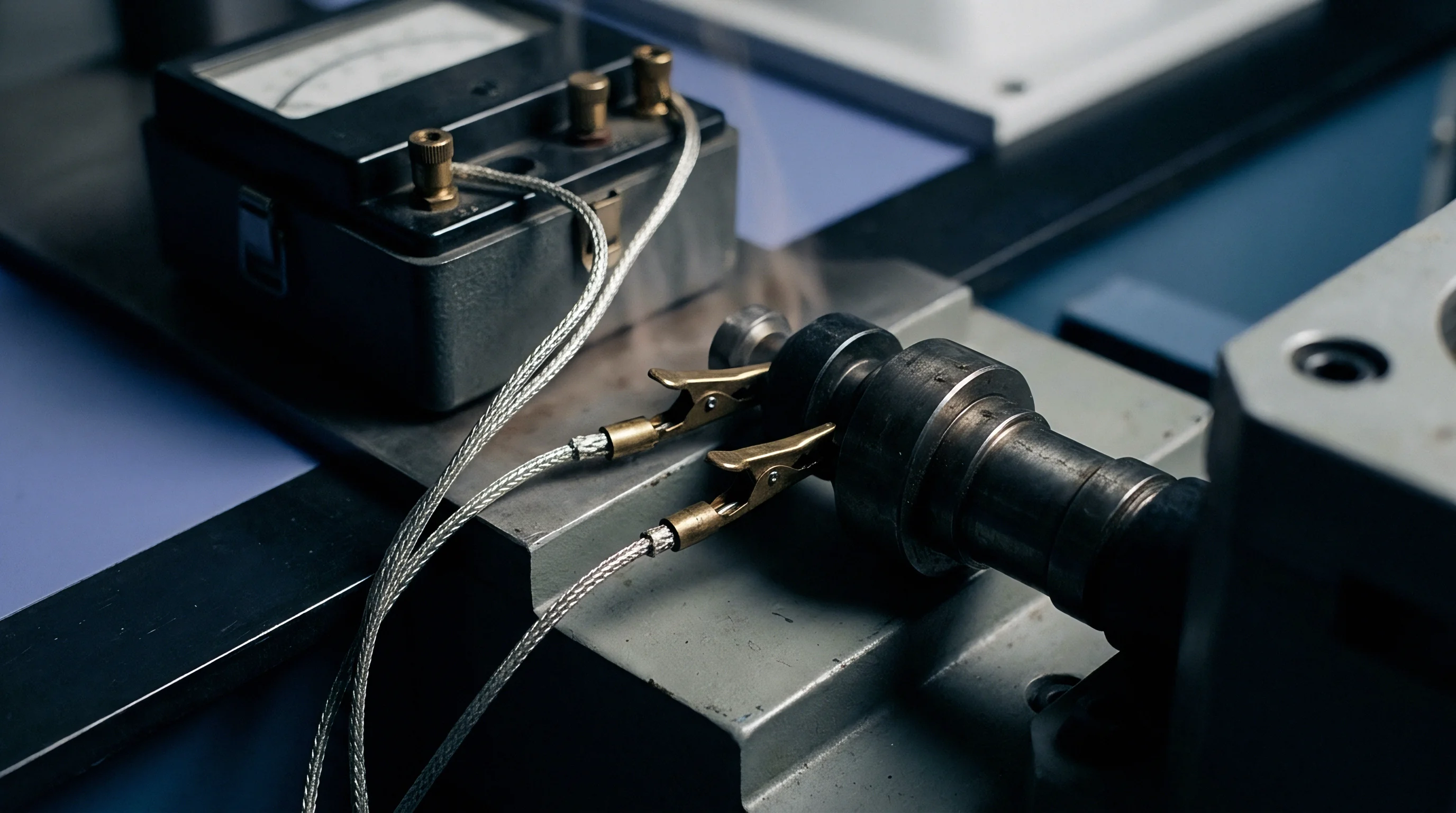
Testing encapsulated sensors properly means separating static calibration errors from transient soak delays. Laboratories operating under ISO/IEC 17025 verify sensors using stirred liquid baths, ice cells, and fixed-point metal freezing cells. Static calibration tracks the probe’s resistance-versus-temperature curve against reference platinum thermometers traceable to national metrology institutes.
Dynamic calibration records time-domain step responses to establish thermal time constants under controlled fluid mechanics.
Uncertainty budgets for dynamic response must cover metrological baselines alongside mechanical plunge timing. The combined standard uncertainty includes the reference thermometer calibration, bath temperature uniformity, bridge linearity, stem conduction, and the plunge actuator’s trigger repeatability. The table below outlines an uncertainty budget for calculating the tau zero point five time constant of an encapsulated process probe.
| Source of Measurement Uncertainty | Standard Uncertainty (s) | Probability Distribution | Sensitivity Coefficient | Uncertainty Contribution (s) |
|---|---|---|---|---|
| Plunge Actuator Timing Mechanism | 0.005 | Rectangular | 1.0 | 0.0029 |
| Fluid Bath Temperature Stability | 0.012 | Normal | 0.8 | 0.0096 |
| Fluid Velocity Variation (1.0 m/s nominal) | 0.035 | Rectangular | 1.2 | 0.0242 |
| Data Acquisition System Sampling Rate | 0.002 | Rectangular | 1.0 | 0.0012 |
| Probe Concentricity and Mounting Geometry | 0.020 | Normal | 1.0 | 0.0200 |
Combining these individual contributions in quadrature gives a combined standard uncertainty of zero point three three seconds. Using a coverage factor of k equals two yields an expanded uncertainty of zero point six six seconds at approximately ninety-five percent confidence. Achieving that precision on the bench requires rigorous control over both bath velocity and insertion timing within accredited limits.
Standard ISO 10012 mandates that measurement equipment shall be calibrated against standards traceable to the International System of Units at specified intervals to guarantee field validity.
Specifying sensor assemblies involves weighing dynamic response against long-term sensor stability under mechanical and chemical plant stresses. Manufacturing options vary significantly, affecting initial price as well as maintenance costs over time. The following technical points need explicit coverage when drafting procurement specifications for fast-response process sensors:
- Sheath Outer Diameter Selection establishes the mechanical strength threshold while defining the minimum achievable thermal mass and basic time constant constraint.
- Potting Material Thermal Conductivity determines internal conductive resistance and prevents air void formation around the primary sensing element.
- Thermowell Insertion Length Ratio minimizes stem conduction errors by ensuring the active sensing zone sits deep within the uniform fluid velocity profile.
- Dual-Element Redundancy Configuration provides parallel signal channels to detect internal potting degradation and drift through continuous cross-comparison.
- Traceable Dynamic Calibration Certificates confirm real-world response times under standardized fluid velocity conditions prior to plant installation.
Procurement documents must specify clear acceptance limits for both static tolerance and step-response timing. Requesting only static tolerance classes under IEC 60751 leaves installations exposed to assemblies with excessive soak delays. Requiring ISO 17025 test documentation guarantees that delivered hardware meets both baseline accuracy limits and dynamic response requirements.

Settlement
Analyzing thermal soak delays in encapsulated sensors highlights the trade-off between structural survivability and response speed. Thicker sheath walls, heavy thermowells, and dense potting protect fragile platinum elements from plant conditions, but every layer adds thermal resistance and heat storage capacity. That protective mass slows heat transfer, distorting control action and hiding critical temperature excursions.
Evaluating temperature assemblies purely on static accuracy ratings inevitably introduces hidden phase lag into real-time feedback loops.
Managing dynamic lag requires an integrated approach to purchasing and verification. Sourcing teams cannot rely on generic datasheet figures; they must require verified time constants tied to documented test conditions. Running incoming checks on sheath fit, potting consistency, and thermowell coupling ensures hardware handles rapid process shifts once installed.
Aligning probe response characteristics with real line kinetics maintains loop stability and preserves plant safety margins over years of operation.