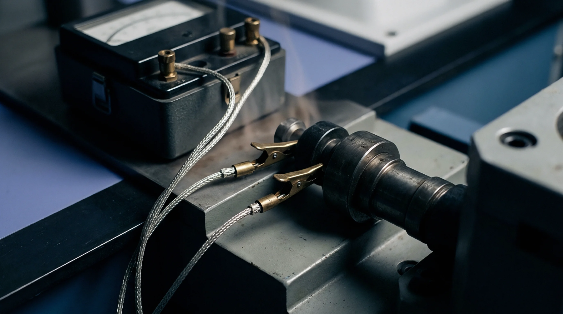
Linear Calibration Coefficient
A scalar constant defines the slope of a direct mathematical relationship between input signal magnitudes and output voltage values within an analog measurement system. Engineers use the linear calibration coefficient to convert raw electrical signals into engineering units like pressure, temperature, or force. This value remains constant only when the sensor behaves in a strictly proportional manner throughout its range.
Non-linearities in the physical transduction process introduce errors that a single coefficient cannot correct alone. Manufacturers derive the constant by performing a least squares regression on a set of reference data points gathered during factory testing. The resulting slope represents the gain of the system under controlled laboratory conditions.
Deviations occur when the thermal environment or mechanical mounting stresses change the sensitivity of the internal strain gauges.
Metrological Verification
Technicians calculate the value by plotting a response curve across the full span of the sensing element. Sensitivity variations originate from batch manufacturing tolerances in the semiconductor substrate. A reference standard exerts known force or physical input while the output signal undergoes precise measurement with a digital multimeter.
Comparison between the theoretical model and the observed data yields the slope value. Thermal drift causes the coefficient to shift over time, necessitating periodic recalibration to maintain the accuracy of the installation. Signal noise or electromagnetic interference can mask the linearity, creating a bias that makes the true slope harder to calculate.
Operators must isolate the measurement chain from external vibration to ensure the captured data reflects the actual input conditions.
Systemic Integration
Applications involving multi-channel data acquisition require consistent slope values across every sensor connected to the same digitizer. Each channel holds a unique register where the software stores the specific scaling factor for that individual input. An incorrect entry in the configuration file produces a systematic offset error that affects every reading generated by the assembly.
Software algorithms multiply the raw count by the stored constant before applying any additive zero correction. This multiplication process happens in real time within the processor unit to output physical units for external display. Hardware changes at the input stage force a total update of the value to keep the data valid for downstream analytics.
Performance Limitation
High-precision instruments require more than a simple constant to account for higher order effects or sensor hysteresis. Saturation at the extreme ends of the measurement range creates a departure from the linearity assumption. A linear calibration coefficient fails to describe the behavior of a sensor that exhibits a curved response profile under high mechanical loading.
Environmental pressure affects the stability of the reference bridge, leading to an erosion of accuracy that the coefficient cannot recover. Complex systems address this by adding a second order polynomial correction factor. The model holds for mid-range operations but lacks the resolution required for highly dynamic signals that fluctuate across the entire input spectrum.
Proper deployment depends on knowing the specific limits where the linear assumption remains valid for the measurement architecture.