State Space Observers for Dynamic Thermal Gradient Mitigation in Sensors
State space thermal observers model internal spatial gradients to eliminate dynamic transient offset errors in sensors during rapid ambient temperature shifts.

Gradient
When ambient temperatures swing rapidly, precision measurement elements develop non-uniform thermal fields across their internal packaging. An external housing thermistor registers the shift immediately, but heat takes time to penetrate the die-attach matrix, ceramic substrate, and silicon proof mass. During a 10 Kelvin per minute thermal ramp, this lag leaves the active transducer die trailing the outer package.
The resulting internal gradients generate localized expansion differentials, thermo-electric offsets, and mechanical strains that an acquisition system cannot distinguish from true measurand changes.
Static thermal compensation relies on steady-state lookup tables or polynomial fits tied to a single temperature sensor, assuming the assembly remains in isothermal equilibrium with its surroundings. Under thermal shock, however, internal temperatures diverge sharply from that single-point measurement. Because a scalar value cannot describe a shifting multi-dimensional heat field, static models leave transient bias shifts entirely uncorrected.
Physical Mechanisms of Dynamic Thermal Errors
Dynamic thermal transients impact physical sensing structures through distinct physical interactions:
- Thermo-mechanical stress imbalance induces localized flexing in silicon MEMS flexures, shifting resonant frequency and zero-rate output baseline in vibrating structure gyroscopes.
- Differential expansion of bond lines causes localized warping across silicon pressure diaphragms, corrupting piezoresistive bridge balance independent of applied fluid pressure.
- Spatial Seebeck potential gradients create parasitic millivolt-level electromotive forces across copper-silicon traces in high-side current measurement shunts, producing false current offsets.
- Substrate thermal capacitance lags alter the optical path length and refractive index of sapphire optical windows in non-dispersive infrared gas absorption chambers, skewing zero-gas calibration curves.
Capturing these dynamic offsets requires testing beyond static polynomial models. Standard calibration profiles hold sensor modules at stepped, isothermal plateaus until internal gradients collapse before logging data ~ an approach that conceals the transient cross-sensitivities typical in aerospace, automotive power systems, and subsea instrumentation. When a device moves from cold storage to full operating power, internal thermal gradients peak within seconds, driving measurement error well outside the steady-state limits listed on the datasheet.
A single temperature sensor mounted on a package housing cannot resolve multi-dimensional spatial heat flux during dynamic thermal transients.
Relying on steady-state lookup tables during thermal transients degrades tracking precision and risks severe signal distortion in closed-loop control loops.

Heat
Conduction through solid sensor assemblies follows Fourier’s law. Rather than solving continuous parabolic partial differential equations on embedded hardware, sensor models discretize the physical geometry into a lumped-parameter thermal network. In this network, thermal capacitances represent the heat storage of discrete structural nodes, while thermal resistances represent conductive heat paths between adjacent nodes and mounting boundaries.
This lumped approach translates continuous heat transport into an equivalent electrical circuit: node voltages correspond to local temperatures, current sources represent heat generated by driver ICs or piezoresistive bridges, and ground represents the heat sink or ambient environment. Observer fidelity depends entirely on setting nodal boundaries along actual thermal conduction paths ~ principally package leads, bond wires, die-attach pads, and encapsulant.

Thermal RC Network Discretization
Constructing the network requires accurate material properties for each layer in the stack. Monocrystalline silicon combines high thermal conductivity with low heat capacity, tracking boundary shifts quickly. By contrast, FR4 circuit boards and epoxy potting compounds conduct poorly while storing substantial heat, functioning as low-pass thermal filters that retard heat penetration.
Each structural element in the package resolves into a discrete node whose thermal resistance and capacitance derive directly from its density, thermal conductivity, and specific heat capacity.
| Material Substrate | Thermal Conductivity (W/m·K) | Specific Heat Capacity (J/kg·K) | Density (kg/m^3) | Node Thermal Resistance (K/W) | Node Thermal Capacitance (J/K) |
|---|---|---|---|---|---|
| Monocrystalline Silicon (100) | 148.0 | 712 | 2330 | 0.45 | 0.0033 |
| Alumina Ceramic (96% Al2O3) | 24.7 | 880 | 3800 | 2.10 | 0.0167 |
| Epoxy Die-Attach (Silver-Filled) | 2.5 | 500 | 3500 | 18.50 | 0.0008 |
| FR4 Substrate (Standard Laminate) | 0.3 | 1200 | 1850 | 85.00 | 0.0444 |
| Kovar Package Frame (Fe-Ni-Co) | 17.3 | 439 | 8360 | 3.80 | 0.0367 |
Assigning nodal boundary conditions accounts for both internal dissipation and external sinks. Heat sources include low-dropout regulators, signal-conditioning ASICs, and optical emitters, while mechanical mounting flanges, harness connectors, and convective air interfaces act as primary heat sinks.
Cauer and Foster Thermal Network Formulations
Thermal RC networks generally follow either a Cauer or a Foster topology. Cauer networks mirror the sensor’s physical layer stack: each node capacitance ties directly to thermal ground, with series resistances joining adjacent layers. Because the nodes align with actual physical interfaces, the calculated states correspond to real temperatures at specific depths inside the package.
Foster networks, by comparison, treat the assembly as a series of uncoupled parallel RC stages fitted to external step-response measurements. While easier to parameterize without internal dimension drawings, Foster nodes have no physical location inside the component. If internal heat dissipation varies independently of boundary temperatures, a Foster model often generates unphysical intermediate states.
Engineers specify Cauer topologies when multi-source heat generation occurs within the package, such as an ASIC heating up adjacent to an unpowered MEMS transducer element.
Cauer thermal network topologies preserve the true physical mapping of internal component heat flow layers.
Deriving node parameters directly from layer geometry provides a sound baseline for state-space observer design.
Matrices
Mapping thermal behavior across n discrete nodes translates directly into linear state-space form. The continuous state equation expresses the derivative of the nodal temperature vector x(t) as a balance of conductive exchanges between nodes, boundary inputs u(t), and internal heat sources.
The continuous state-space linear system takes the canonical mathematical representation:
dotx(t) = A x(t) + B u(t)
y(t) = C x(t) + D u(t)
Here, x(t) in mathbbRn represents the internal node temperatures, u(t) in mathbbRm contains boundary temperature measurements and internal power inputs, and y(t) in mathbbRp holds the estimated temperature gradients driving sensor offset. Matrix A in mathbbRn × n contains the conductance and capacitance coefficients that dictate inter-node dynamics, while matrix B in mathbbRn × m routes boundary conditions and power dissipation into the respective nodes.

Constructing System Matrices from Thermal Physics
Constructing state matrix A requires applying Kirchhoff’s thermal current law at each interior node i. For an interior node i bounded by nodes i-1 and i+1, the continuous balance of heat flux yields:
Ci fracdTidt = fracTi-1 – TiRi-1,i + fracTi+1 – TiRi,i+1
Dividing through by nodal capacitance Ci isolates the state derivative dotTi on the left side of the equation:
dotTi = frac1Ri-1,i Ci Ti-1 – left( frac1Ri-1,i Ci + frac1Ri,i+1 Ci right) Ti + frac1Ri,i+1 Ci Ti+1
For one-dimensional heat flow, matrix A is tridiagonal, sign-symmetric, and strictly negative-definite, guaranteeing asymptotic thermal stability. Output matrix C extracts the internal temperature differences ~ such as Δ Tgradient = Tdie – Tsubstrate ~ that scale the physical sensor offset calibration matrix.

Discretization for Digital Embedded Systems
Because embedded microcontrollers execute state observers at discrete sample intervals Ts, continuous matrices A and B must be discretized. Applying a zero-order hold assumes boundary inputs remain constant over each interval Ts.
The exact matrix exponential conversions follow standard digital control transformations:
Ad = eA Ts = Φ(Ts)
Bd = left( int0Ts eA τ dτ right) B = A-1 (Ad – I) B
Evaluating matrix exponentials via Taylor series on fixed-point hardware introduces truncation errors when Ts approaches the smallest thermal time constant τmin = Rmin Cmin. Systems therefore compute Ad off-line or during system initialization using Padé approximations, preserving numerical stability across the full operating range.
State Form Conversion Checklist
Transforming continuous thermal models into real-time state matrices demands a structured implementation procedure:
- Derive physical node thermal capacities from material density, specific heat, and geometric volume definitions.
- Calculate conductive thermal resistances between geometric node centers using boundary cross-sectional areas.
- Assemble continuous matrix A by placing nodal heat conduction loss sums along the main diagonal.
- Define input matrix B to route boundary sensor inputs and internal power dissipation channels to target nodes.
- Compute discrete system matrix Ad using exact matrix exponentials scaled to target sample rate Ts.
- Validate matrix eigenvalue stability by confirming all discrete matrix eigenvalues sit strictly within the unit circle.
Per ISO 26262 functional safety clauses, dynamic compensation firmware embedded in automotive safety sensors must demonstrate deterministic matrix calculation execution bounds.
Discretizing continuous matrices without verifying eigenvalue locations risks numerical instability whenever rapid ambient transitions excite high-frequency spatial modes in the network.
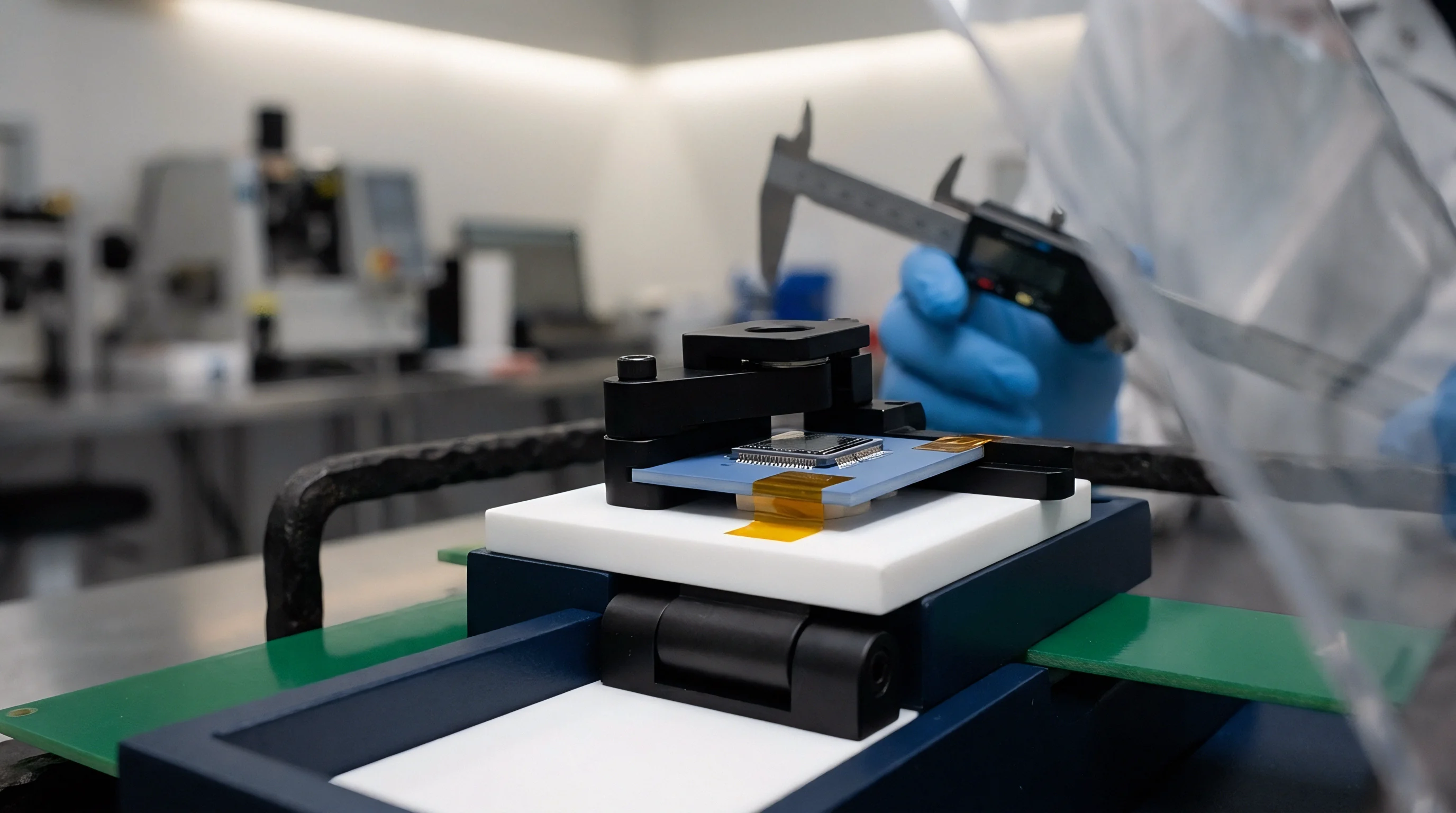
Observer
Direct temperature sensing at every internal package node is rarely practical. Board layouts place thermistors on external PCB copper or read junction diodes embedded in signal ASICs, leaving the primary sensing die unprobed. A dynamic state space observer estimates the complete unmeasured internal nodal temperature vector hatx(k) using only available boundary temperature measurements ym(k) and system input vector u(k).
The observer runs a real-time plant model corrected by a feedback term that scales the discrepancy between actual boundary readings ym(k) and estimated boundary states haty(k) = Cm hatx(k).
Luenberger Observer Dynamics
The discrete-time Luenberger state space observer computes updated thermal state estimates at each sample frame k according to the difference equation:
hatx(k+1) = Ad hatx(k) + Bd u(k) + L left( ym(k) – Cm hatx(k) right)
Gain matrix L in mathbbRn × p dictates how quickly estimation errors collapse. Subtracting the observer state equation from the true physical state equation yields the state estimation error dynamics e(k) = x(k) – hatx(k):
e(k+1) = (Ad – L Cm) e(k)
The eigenvalues of (Ad – L Cm) govern error decay rates. For the estimation error to converge asymptotically to zero, gain matrix L must place all eigenvalues of (Ad – L Cm) strictly inside the unit circle on the complex z-plane.
Thermal Observability Verification
Synthesizing gain matrix L requires that the thermal model satisfy the Kalman observability criterion. The observability matrix mathcalO is constructed from measurement matrix Cm and discrete state matrix Ad:
mathcalO = beginbmatrix Cm \ Cm Ad \ Cm Ad2 \ vdots \ Cm Adn-1 endbmatrix
When mathcalO has full rank n, the boundary thermistors provide adequate thermal coupling to reconstruct all internal node temperatures from boundary data alone.
Kalman Filtering for Thermal Disturbances
When air turbulence or electrical pickup injects stochastic noise into boundary thermistor readings, a discrete Kalman filter replaces the fixed Luenberger gain L with a time-varying optimal gain K(k), minimizing state estimation error covariance against process noise covariance Q and measurement noise covariance R.
| Observer Topology | Convergence Time (s) | Peak Gradient Error (K) | Steady-State Residual Noise (K) | MCU Execution Time (us) | Memory Overhead (Bytes) |
|---|---|---|---|---|---|
| Static Polynomial (Baseline) | Infinite (Lags) | 4.85 | 0.02 | 1.2 | 128 |
| Luenberger Observer (Deadbeat Poles) | 0.45 | 0.62 | 0.38 (Amplified) | 12.4 | 512 |
| Luenberger Observer (Optimal Poles) | 2.10 | 0.28 | 0.08 | 12.4 | 512 |
| Discrete Kalman Filter (Steady-State K) | 1.80 | 0.14 | 0.03 | 18.6 | 1024 |
| Extended Kalman Filter (Temperature-Dependent R, Q) | 1.40 | 0.05 | 0.02 | 84.2 | 3072 |
Process covariance Q accounts for uncertainties in thermal conductivities, packaging densities, and internal power dissipation, while measurement covariance R captures ADC quantization and thermistor noise floors. The ratio Q/R balances filter responsiveness against noise rejection: higher ratios cause the filter to track boundary measurements more aggressively during thermal transitions, but pass more high-frequency noise into the estimated gradient.
Under a 10 K/min dynamic ramp, an Extended Kalman Filter reduces internal thermal gradient estimation error to 0.05 K, compared to 4.85 K for static polynomial lookup tables.
Temperature-dependent non-linearities in die-attach adhesives can degrade observer stability when thermal sweeps span wide ranges from -40 to +125 degrees Celsius.
Validation
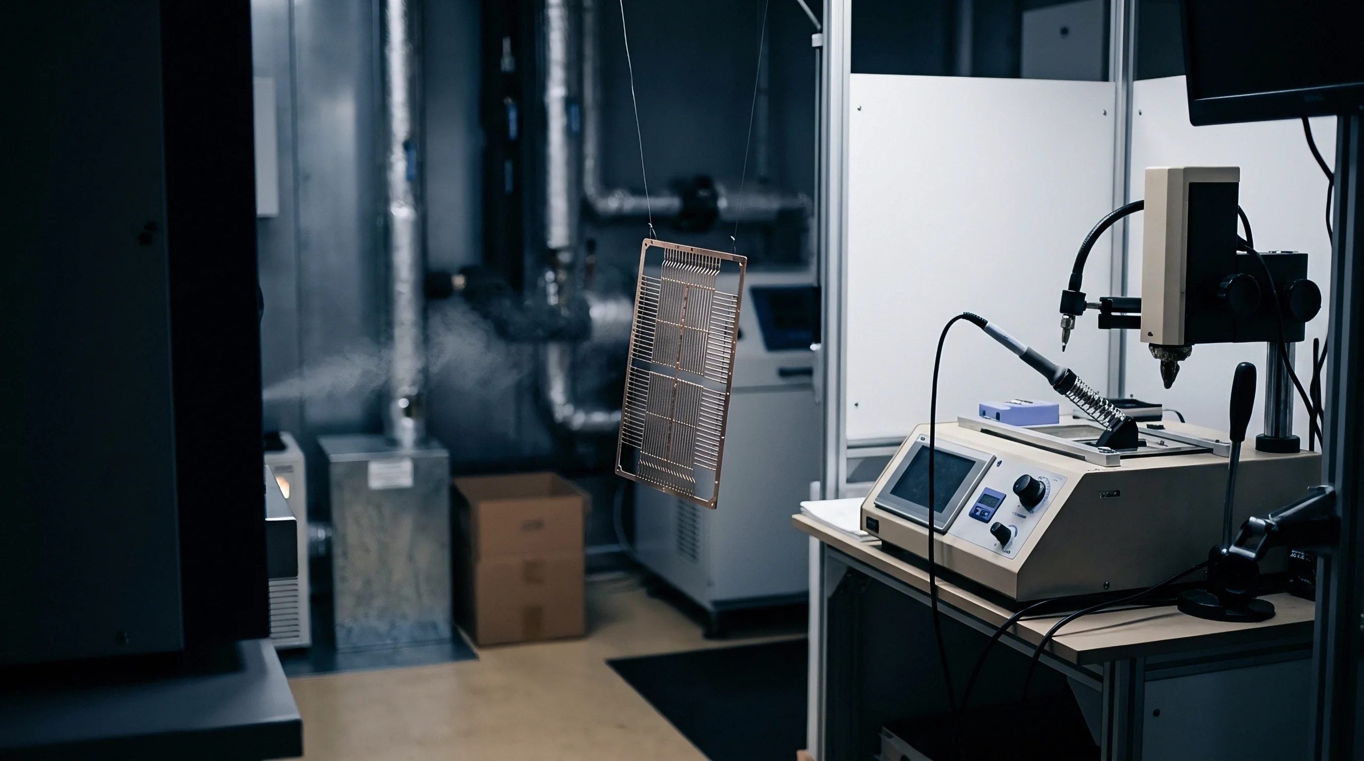
Validating dynamic thermal observers requires transient testing rather than static soak plateaus. Test bench setups require high-bandwidth Peltier thermal pulse plates, infrared thermography imaging, and multi-channel high-speed thermal logging hardware capable of sampling at rates faster than the smallest internal thermal time constant.
Model validation subjects the sensor housing to controlled heat flux pulses while logging actual transducer drift against observer predictions. Calibrated thermal imaging cameras capture spatial surface fields through optical chambers, providing reference spatial temperature distributions to validate lumped state node predictions.

Bench Execution Protocol
Validating dynamic state observers requires a precise step-by-step physical test sequence:
- Mount the sensor under test to a temperature-controlled peltier plate inside a nitrogen-purged thermal enclosure.
- Connect internal raw transducer output signals and auxiliary thermistor channels to a synchronized 24-bit data acquisition system sampling at 100 Hz.
- Apply a thermal step pulse from 25 to 85 degrees Celsius at a ramp rate exceeding 15 Kelvin per minute.
- Record uncompensated sensor output drift, boundary thermistor measurements, and real-time state observer output predictions simultaneously.
- Inject mathematical thermal state estimates into the sensor output signal conditioning chain to compute corrected measurement values.
- Compare residual dynamic offset error against steady-state baseline performance specifications across five consecutive thermal sweep cycles.
Where Do Thermal State Observer Models Break Down?
Observer accuracy drops when actual assembly interfaces diverge from modeled parameters. Interface resistance between a sensor package and its PCB pad varies with fastener torque, solder voiding, and thermal interface material degradation. Large voids beneath a driver ASIC, for example, redirect heat flow and can alter local thermal resistance by up to 30 percent relative to nominal values.
Uncontrolled convection creates further divergence. Forced air cooling across an unshielded sensor housing alters external thermal resistance dynamically based on airflow velocity, changing boundary input matrix B without triggering onboard thermistors. When internal heat paths alter due to mechanical delamination or solder cracking, fixed observer matrices Ad overestimate internal heat diffusion rates, leaving uncompensated transient offsets.
Transient thermal shocks induce mechanical strain, yet component datasheets define only steady-state isothermal performance, leaving dynamic gradient compensation to system integrators.
Provision
Executing state-space observers in commercial sensor designs requires balancing algorithm complexity against limited compute resources. Microcontrollers managing the signal chain operate under rigid budgets for power, RAM, and interrupt latency. Adding matrix multiplication to primary ADC acquisition routines means aligning model size directly with available hardware resources.
Entry-level 32-bit ARM Cortex-M0+ and 16-bit controllers lack hardware floating-point support. Emulating double-precision operations in software inflates interrupt execution times and risks missing ADC conversion deadlines. For these targets, designers scale matrices into Q15 or Q31 fixed-point formats to complete observer updates within standard timer interrupts.

Microcontroller Computational Resource Demands
Execution cost scales quadratically with state dimension n. Matrix-vector multiplication within state update step hatx(k+1) = Ad hatx(k) + Bd u(k) + L e(k) requires n2 + n · m + n · p floating-point multiplications per execution cycle. For a 5-node thermal observer with 2 inputs and 1 measurement, each update demands 40 scalar multiplications and 35 additions.
| Processor Core Architecture | State Vector Size (n) | Data Format Topology | Cycles Per State Update | Execution Time at 48 MHz (us) | Flash Memory Footprint (KB) |
|---|---|---|---|---|---|
| ARM Cortex-M0+ (No FPU) | 3 Nodes | 32-bit Fixed-Point (Q31) | 420 | 8.75 | 2.4 |
| ARM Cortex-M0+ (No FPU) | 5 Nodes | 32-bit Floating-Point (Soft) | 3850 | 80.20 | 6.8 |
| ARM Cortex-M4F (Single FPU) | 5 Nodes | 32-bit Floating-Point (Hard) | 310 | 6.45 | 3.8 |
| ARM Cortex-M4F (Single FPU) | 8 Nodes | 32-bit Floating-Point (Hard) | 760 | 15.83 | 5.2 |
| ARM Cortex-M7F (Double FPU) | 8 Nodes | 64-bit Floating-Point (Hard) | 280 | 2.67 | 8.1 |
Selecting processors with hardware floating-point units, such as the ARM Cortex-M4F, eliminates fixed-point scaling steps and removes the risk of integer overflow during steep thermal transitions.
Commercial Sourcing and Specification Strategies
Specifying sensors for dynamic thermal environments requires looking beyond standard parametric tables to evaluate how vendors qualify transient behavior. Advanced module suppliers integrate internal thermal state observers directly into their sensor DSP firmware, delivering dynamically compensated measurement streams over SPI or I2C interfaces.
When sourcing discrete transducer dies or raw packages, procurement specifications must define dynamic qualification requirements explicitly, establishing maximum permissible offset drift under stated thermal ramp rates instead of relying on isothermal accuracy bands.
Supply agreements require detailed packaging thermal characterization dossiers to establish baseline parameters for downstream observer matrices.
Component supply contracts for mission-critical sensing modules must include dynamic thermal ramp test clauses defining maximum allowable transient zero-point drift under a specified Kelvin-per-minute thermal rate.