Statistical Acceptance Sampling for Incoming Transducer Lot Quality Audits
Variable acceptance sampling under ANSI ASQ Z1.9 reduces sample size by 70 percent while enforcing strict consumer risk bounds on transducer lot audits.


Dock
Receiving shipments of industrial pressure transducers and strain-gauge load cells exposes operations to latent defects before electrical bench checks even begin. When a sensor lot arrives at the bay, statistical quality control transforms factory tolerance claims into empirical audit records. Freight vibration, thermal cycling inside containers, and handling shocks routinely shift baseline zero balances and internal strain states.
A thorough audit starts on the loading pad with structured physical inspection, environmental triage, and sample selection drawn from statistical lot tables. Skipping intake protocol risks sending units to assembly lines with diaphragms, sensing elements, or internal electronics damaged during transit.
Physical inspection starts at the outer cartons and ESD packaging, checking for structural damage, triggered humidity indicators, or broken seals. High-precision transducers built with thin-film strain gauges or piezoresistive silicon dies rely on intact hermetic seals to isolate bridge circuits from atmospheric moisture. When crates arrive showing water exposure or crushed corners, housing stress relief can shift zero-point calibration before a unit ever sees line pressure.
Inspectors evaluate external connectors, cable gland strain reliefs, threads, and mounting flanges for dimensional fit and transit damage. Threaded fittings ~ like standard NPT or BSPP connections ~ are verified with thread pitch gauges to ensure burrs or galled threads won’t block proper torquing on the bench.
Unchecked transducer drift compromises baseline accuracy across downstream testing systems.
Valid statistical sampling relies on lot homogeneity. A shipment cannot be treated as a uniform population if it merges multiple production runs, different silicon wafer diffusion batches, or separate resistor trimming cycles. Inspectors review vendor paperwork, outer labels, and serial number sequences to verify that incoming units come from a single manufacturing lot.
Combining sub-lots within one audit distorts standard deviation calculations and introduces bimodal distribution curves during parametric testing. If paperwork reveals split production lots or multiple factory calibration dates in one shipment, receiving divides the delivery into distinct sub-lots and samples each batch on its own.

Physical Intake Verification and Packaging Stress
Mechanical verification confirms housing integrity and connector pin layout before applying excitation voltage. Technicians check pin assignments against vendor drawings using pinout templates to avoid short circuits on the test bench. Loose shells, missing O-rings, or bad potting at cable terminations signal vendor quality gaps that correlate directly with IP67 or IP68 field failures.
On stainless steel diaphragm transducers, optical inspection under low-power stereomicroscopes uncovers surface scratches, weld spatter, or minor dents that create local stress risers and non-linear output under pressure cycling.
Bypassing thermal stabilization leads to transient errors during initial electrical testing.
Sensors require environmental conditioning before electrical testing. Units pulled from unheated freight holds or cargo holds carry thermal gradients that shift zero balance and induce temporary drift. Unpacking cold units directly inside a climate-controlled calibration lab causes condensation on internal circuits and shifts silicon strain gauge resistance.
Intake protocols require a thermal stabilization soak in the test facility, typically lasting between six and twenty-four hours depending on sensor thermal mass. Skipping this hold distorts baseline zero readings, causing false lot rejections for vendor offset errors when the real culprit is thermal lag.
| Defect Category | Specific Failure Mode | Inspection Method | Acceptance Threshold | Action Upon Non-Conformance |
|---|---|---|---|---|
| Packaging Integrity | Humidity card color shift above 30 percent RH | Visual check at package opening | Zero instances per lot | Quarantine lot; require vendor dry-bake certification |
| Mechanical Flange | Galled threads or flange face scratches | Optical comparator and thread gauge | Zero major defects; max 1 minor scratch | Reject unit; sample expansion for lot thread engagement check |
| Connector / Pinout | Misaligned pins or loose potting seal | Mechanical pin template check | Zero defect allowance | Return lot for connector rework |
| Diaphragm Condition | Diaphragm pitting, denting, or weld flash | Stereomicroscope 10x magnification | Zero surface defects on sensing area | Immediate lot rejection under critical defect classification |
| Documentation | Missing factory calibration certificate or batch trace | Document reconciliation | 100 percent paperwork compliance | Hold lot in receiving quarantine pending paper trace delivery |

Stratified Batch Sampling at Receiving
Pulling samples from incoming pallets demands systematic random selection across the entire container volume. Instead of taking boxes solely from top layers, inspectors follow a stratified map to select samples from top, middle, bottom, front, and rear positions. Sampling bias on the dock lets localized defects ~ such as cartons damaged against container walls ~ escape notice or distort variance calculations.
Every selected unit receives a unique audit tracking label to track chain of custody through zero balance checks, full-scale output measurements, and hysteresis screening.
A temperature drop of 15 °C during air transit shifts uncompensated zero offset by 0.42 % of full scale span in unsealed piezoresistive transducers.
Sample sizes depend on overall lot volume and risk thresholds defined in quality agreements. Using standardized sampling tables maintains statistical rigor without slowing dock operations. Receiving inspectors match carton counts against packing slips, verify heat numbers or lot codes stamped on housing bodies, and log the shipment into receiving quarantine within the ERP platform.
Until statistical sampling satisfies physical and metrological audit criteria, the inventory system blocks movement to production, keeping unverified units off assembly lines.

Environmental Conditioning and Thermal Stabilization
Equalizing temperature across internal transducer assemblies requires controlled storage before electrical measurement. Stainless steel housings with oil-filled sensing cavities have thermal time constants dictated by oil volume and internal heat paths. Bringing cold sensors into a 23 °C laboratory triggers thermal expansion of the fill oil, causing temporary pressure spikes against the silicon diaphragm.
Testing during this transient phase yields false zero-offset readings that shift until internal temperatures balance out.
Unpacking procedures require placing individual transducers on wire-mesh racks that allow uniform airflow around each housing. Laboratory temperature during stabilization must stay within 23 °C ± 1.0 °C, with relative humidity held below 50 percent to prevent moisture films on ceramic substrates or glass-to-metal header seals. Technicians log ambient temperature and relative humidity at the start and end of the soak using calibrated environmental monitors traceable to national metrology standards.
Only after completing the documented soak window does the sample lot move to the calibration bench for zero-point and full-scale output audits.

Visual and Mechanical Defect Taxonomies
Categorizing defects caught during receiving clarifies vendor feedback and gives structure to supplier rating calculations. Critical defects involve physical non-conformances that leave a sensor unsafe or inoperable, such as cracked housings, crossed pins, or ruptured diaphragms. Major defects degrade measurement performance beyond specification limits, including zero offsets past declared tolerances or out-of-spec mounting threads.
Minor defects cover cosmetic flaws, slightly misaligned labels, or small surface scratches that do not impact mechanical or electrical operation.
Audit personnel log visual and mechanical defects on intake sheets, grading each flaw against drawing requirements and purchasing specifications. A single critical defect triggers immediate rejection of the entire lot without further electrical testing. Major defect counts feed directly into attribute acceptance calculations, where exceeding the assigned Acceptable Quality Limit prompts lot quarantine and vendor escalation.
Tracking visual defect categories over successive shipments exposes recurring supplier process issues, like tool wear on machining lines or inadequate cleaning before packaging.
Transit temperature swings outside historical averages can induce baseline zero shifts prior to package unsealing.


Calculus
Statistical modeling for lot acceptance relies on clear boundaries between allowable defect rates and population drift. When auditing incoming transducer shipments, quality engineering teams choose between attribute and variable sampling schemes based on sample size limits, unit testing costs, and the parametric nature of the data. Attribute sampling evaluates components on a binary pass-fail basis by counting non-conforming units.
Variable sampling measures continuous parametric data, using the sample mean and standard deviation to estimate the portion of the population exceeding specification limits.
Attribute sampling schemes under standards like ANSI/ASQ Z1.4 work well for quick visual checks or simple continuity tests. But in transducer audits where every run requires precision pressure cycles, thermal stabilization, and automated voltage readings, attribute sampling demands large sample sizes for high confidence. Calibrating eighty or one hundred twenty-five transducers per lot on high-accuracy pressure benches imposes heavy labor overhead.
Variable sampling plans under ANSI/ASQ Z1.9 leverage continuous data to offer equivalent statistical confidence with far smaller sample sizes, making them the practical choice for precision sensor qualification.
Evaluating lots solely through binary attribute limits obscures critical parametric safety margins.
Variable sampling assumes that measured sensor parameters ~ like zero offset voltage, full-scale span, or thermal zero shift ~ follow a normal Gaussian distribution across the manufacturing lot. Technicians measure the parameter on each sample unit, calculating the sample mean barX and standard deviation s. These metrics determine upper and lower quality statistics, QU and QL, which represent the distance from the sample mean to upper and lower specification limits in units of standard deviation.
Comparing QU and QL against critical acceptance values k from standard sampling tables establishes whether the lot passes statistical audit.

Attribute versus Variable Sampling Schemas
Choosing the mathematical framework for incoming lot audits directly shapes laboratory throughput and false acceptance risks. Attribute plans flag a transducer as non-conforming if its zero-point offset strays even 0.01 percent beyond the specified ± 0.10 percent full scale output limit. This binary cutoff discards valuable margin data; a unit missing tolerance by 0.001 percent carries the exact same weight as one off by 1.0 percent.
Attribute sampling cannot differentiate between a tightly grouped population sitting near a tolerance limit and a widely dispersed lot spread across specification boundaries.
In variable sampling schemes, calculated standard deviation determines overall lot acceptance.
Variable sampling gets far more information from every tested unit by capturing exact numerical deviations from target nominal values. A lot with a tight distribution centered on nominal output passes audit criteria with small sample sizes ~ often just five to fifteen units from a shipment of five hundred transducers. If supplier processes suffer from tool wear, bath temperature variations, or resistor batch differences, the sample standard deviation s expands quickly.
The calculated quality statistic then drops below the critical threshold k, triggering lot rejection even if every individual unit in the audit sample sits inside published tolerance limits.
| Evaluation Parameter | ANSI/ASQ Z1.4 (Attribute Plan) | ANSI/ASQ Z1.9 (Variable Plan) | Operational Advantage |
|---|---|---|---|
| Sample Size (Normal Level II, AQL 1.0) | 50 units per lot | 15 units per lot | 70 percent reduction in bench calibration time |
| Measurement Data Required | Binary pass/fail classification | Continuous numerical output (mV/V or mA) | Captures population distribution spread and mean shift |
| Underlying Distribution Assumption | Distribution-free (binomial/Poisson) | Normal (Gaussian) distribution required | Variable requires normality verification before use |
| Sensitivity to Process Drift | Detects drift only after tolerance breach | Detects standard deviation expansion early | Provides advance warning of vendor process instability |
| Bench Execution Time per Lot | Approx 8.5 hours (10 min/unit) | Approx 2.5 hours (10 min/unit) | Saves 6.0 technician bench hours per incoming lot |

Can Variable Sampling Lower Audit Costs for Small Transducer Batches?
Using variable acceptance sampling for small incoming sensor lots reduces test time while keeping consumer risk low. When receiving high-value pressure transducers or custom load cells in small quantities between twenty and one hundred units, attribute sampling forces technicians to test a large fraction of the shipment. Variable sampling plans under ANSI/ASQ Z1.9 Special Inspection Levels S-3 or S-4 allow quality engineers to evaluate lots with sample sizes as small as three to five units, assuming historical vendor data confirms normal distribution behavior.
Savings come from shorter calibration setups, reduced wear on master reference standards, and faster lot turnaround through receiving quarantine. Testing five transducers through a five-point calibration cycle takes about one hour on an automated pressure manifold, while an attribute sample of thirty-two units ties up the bench for over five hours. The reduced technician hours and equipment time easily outweigh the upfront effort needed to configure variable sampling templates and normality verification scripts.

Acceptable Quality Limit and Consumer Risk Boundaries
Setting the Acceptable Quality Limit (AQL) and Lot Tolerance Percent Defective (LTPD) establishes the contractual risk boundaries between supplier and buyer. The AQL represents the maximum percentage of non-conforming units a buyer accepts as a long-term process average. Operating Characteristic (OC) curves plot the probability of lot acceptance Pa against the actual non-conforming fraction p in a submitted lot.
A standard AQL of 0.4 percent at Normal Inspection Level II yields a high acceptance probability ~ typically 95 percent (1 – α = 0.95) ~ when vendor defect rates stay under 0.4 percent.
Consumer risk β marks the probability of accepting a defective lot whose defect rate meets or exceeds the LTPD limit, typically benchmarked at a 10 percent acceptance probability (Pa = 0.10). In high-reliability applications ~ like pressure sensors for automotive safety testing or industrial boiler controls ~ accepting a lot with 2.0 percent non-conforming units poses genuine operational hazards. The variable sampling math selects sample size n and critical distance k so the OC curve drops sharply between AQL and LTPD, protecting the buyer from accepting drifting supplier lots.
Standard audit protocols fix producer risk at five percent while keeping consumer risk below ten percent across sensor lots.

Stepwise Operational Sequence for Variable Lot Acceptance
Executing a variable acceptance sampling audit follows a step-by-step mathematical routine to calculate parametric quality statistics against specification limits.
- Draw a random sample of n transducers from the incoming shipment according to the ANSI/ASQ Z1.9 sample size code letter derived from lot size and specified inspection level.
- Condition all sample units in the temperature-controlled laboratory environment for the specified thermal stabilization window.
- Mount each sample transducer on the calibration manifold and record zero-point output voltage Vzero and full-scale output voltage VFS under reference environmental conditions.
- Calculate the individual parametric performance metrics, such as full-scale span S = VFS – Vzero or zero offset percentage Ezero = (Vzero / Vsupply) × 100.
- Compute the sample mean barX = frac1nsumi=1n Xi for each evaluated parameter across the n sample units.
- Calculate the sample standard deviation s = sqrtfrac1n-1sumi=1n (Xi – barX)2 to measure population spread.
- Compute the upper quality statistic QU = fracUSL – barXs and the lower quality statistic QL = fracbarX – LSLs, where USL and LSL represent upper and lower specification boundaries.
- Compare the smaller of QU or QL against the critical accept factor k retrieved from the standard ANSI/ASQ Z1.9 table for the specified sample size and AQL; if the calculated quality statistic exceeds or equals k, release the lot, otherwise transfer the lot to quarantine rejection status.
ANSI ASQ Z19 Clause 23 mandatory switching rules automatically escalate sampling inspection to tight levels when two consecutive lots reveal standard deviation expansion beyond baseline historical variance.
Normality of data must be confirmed before applying variable sampling math. If vendor processes experience tool shifts, dual-cavity mold differences, or mixed material lots, measured values may show skewness or kurtosis that breaks Gaussian assumptions. Quality software runs Shapiro-Wilk or Anderson-Darling normality tests on sample datasets before calculating QU and QL.
If sample data fails normality testing at a significance level of α = 0.05, the variable protocol aborts and shifts to an equivalent ANSI/ASQ Z1.4 attribute plan.
When measurement uncertainty exceeds sample variance, sampling plan calculations break down into noise.

Probe
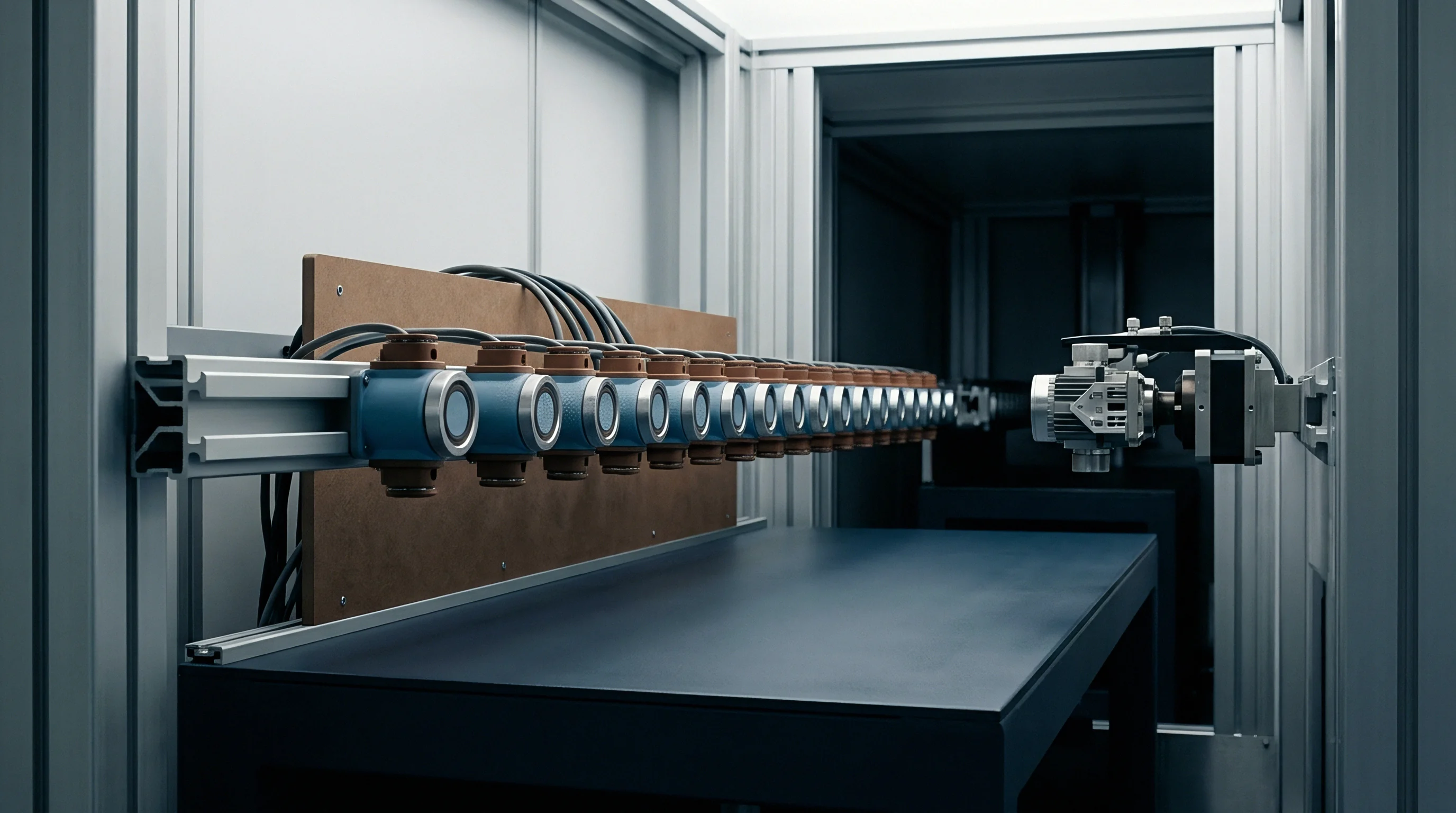
Testing electrical outputs over multi-point pressure cycles requires isolating environmental variables from intrinsic sensor non-linearity. Bench testing incoming transducer samples requires high-accuracy reference instruments, automated pressure controllers, and stable excitation power supplies that add negligible uncertainty to audit measurements. Standard metrology practice requires that calibration equipment uncertainty stay well below the tolerance band of the sensor under test.
Maintaining a Test Uncertainty Ratio (TUR) of at least 4:1 ~ and ideally 10:1 ~ prevents bench system noise from masking vendor manufacturing defects or driving false rejections.
Bench testing starts with power supply stability and signal conditioning checks. Piezoresistive strain gauge bridges and unamplified millivolt-output transducers react directly to changes in excitation voltage; an uncompensated 0.05 percent fluctuation in excitation voltage creates an immediate 0.05 percent shift in output signal. Precision DC power supplies on audit benches maintain voltage regulation within ± 0.005 percent across eight-hour shifts, monitored continuously by digital multimeters at transducer input terminals.
Signal conditioning channels use high-resolution 24-bit analog-to-digital converters with low thermal drift to detect microvolt variations during pressure steps.
Unexpected zero shifts indicate latent stress or deformation within the diaphragm structure.
Pressure generation relies on automated deadweight testers or digital pressure controllers fitted with quartz Bourdon tube reference transducers. When testing a 0 to 10 bar pressure transducer rated at ± 0.1 percent full scale accuracy, the controller’s total expanded uncertainty cannot exceed ± 0.025 bar across its entire operating range. Calibration manifolds run on non-contaminating nitrogen gas or clean hydraulic oil, using fast-acting isolation valves and volume controllers to hold target pressures stable within ± 0.002 bar during measurement windows.

Bench Infrastructure and Reference Standards
Traceability connects incoming laboratory measurements back to national metrology institutes like NIST or PTB. Calibration certificates for reference pressure monitors must show active ISO/IEC 17025 accreditation stamps, stated coverage factors (k = 2 for 95 percent confidence), and documented calibration interval histories. Allowing reference standards to pass their re-calibration due dates undermines the legal and metrological validity of incoming lot rejections, leaving the buyer vulnerable during commercial disputes.
Thermal variation introduces additional variance components into combined uncertainty calculations.
During bench verification, technicians track zero offset drift over a continuous forty-eight-hour stabilization period. Laboratory environmental systems maintain ambient air temperature within 23 °C ± 0.5 °C and relative humidity within 45 percent ± 5 percent. Temperature sensors attached directly to the transducer body track thermal shifts caused by gas expansion inside high-pressure manifolds.
Rapid pressurization cycles cause localized adiabatic cooling that drops sensor body temperature by several degrees Celsius; taking readings before thermal equilibrium restores introduces systematic offset errors that distort non-linearity calculations.
| Uncertainty Component Source | Standard Uncertainty ui | Probability Distribution | Sensitivity Coefficient ci | Uncertainty Contribution ui(y) |
|---|---|---|---|---|
| Primary Pressure Standard Accuracy | 0.0020 bar | Normal (k = 2) | 1.0 | 0.00100 bar |
| Pressure Controller Stability & Resolution | 0.0008 bar | Rectangular | 1.0 | 0.00046 bar |
| Digital Multimeter Voltage Measurement | 0.00005 mV | Normal (k = 2) | 0.1 bar/mV | 0.0000025 bar |
| Excitation Power Supply Regulation | 0.00010 V | Rectangular | 1.0 bar/V | 0.000058 bar |
| Ambient Thermal Drift (± 0.5 °C) | 0.29 °C | Rectangular | 0.002 bar/°C | 0.000580 bar |
| Transducer Mounting Torque Variation | 0.0003 bar | Rectangular | 1.0 | 0.000173 bar |
| Repeatability (Standard Deviation of 5 Runs) | 0.0007 bar | Normal (n = 5) | 1.0 | 0.000700 bar |
| Combined Standard Uncertainty uc = sqrtsum ui(y)2 = 0.00147 bar | Expanded Uncertainty U = 2 × uc = 0.00294 bar (0.0294 % FS) | ||||

Metrological Uncertainty Propagation in Verification
Calculating combined measurement uncertainty follows the Guide to the Expression of Uncertainty in Measurement (JCGM 100:2008 GUM) framework. Every individual contributor to error ~ reference standard calibration uncertainty, multimeter resolution, thermal fluctuations, pressure stability, and mounting strain ~ is quantified as a standard uncertainty ui. Combining these values in quadrature produces the combined standard uncertainty uc, which is then multiplied by coverage factor k = 2 to yield the expanded uncertainty U at approximately 95 percent confidence.
When evaluated expanded uncertainty U reaches 0.00294 bar on a transducer with a specified tolerance of ± 0.010 bar, the Test Uncertainty Ratio calculates to 0.010 / 0.00294 = 3.4:1. Although a 3.4:1 ratio approaches standard industry targets, guardbanding rules under ISO 14253-1 require narrowing acceptance limits by the expanded measurement uncertainty value. Guardbanding reduces the acceptance boundaries from ± 0.010 bar down to ± 0.00706 bar, protecting the buyer from accepting non-conforming units that land near tolerance edges because of test system noise.

Hysteresis Non-Linearity and Zero Wander Analysis
Multi-point pressure verification runs a five-point or nine-point ascending and descending pressure loop to measure sensor hysteresis and non-linearity. Test software commands the pressure controller in equal steps: 0 percent, 25 percent, 50 percent, 75 percent, 100 percent, and back down through 75 percent, 50 percent, 25 percent, to 0 percent of full scale span. Dwell time at each pressure step allows mechanical stress in the sensor body to settle before recording output voltage.
Hysteresis represents the maximum difference between ascending and descending output readings recorded at the same applied pressure level, expressed as a percentage of full scale output:
Hmax = fracmax|Vascend – Vdescend|VFS – Vzero × 100
Best Fit Straight Line (BFSL) non-linearity measures the maximum deviation of ascending and descending points relative to a linear regression line fit to the calibration dataset. Some vendor specifications quote End-Point non-linearity, which draws a straight line strictly between zero and full-scale output points. End-point calculations usually yield higher non-linearity values than BFSL methods; incoming audit software must apply the exact non-linearity formula stated in vendor specifications to avoid invalid lot rejections.

Physical Mechanisms of Early Drift Failures
Analyzing physical failure modes caught during incoming bench audits reveals structural weaknesses in vendor design or manufacturing processes.
- Adhesive creep at strain gauge boundary causes continuous negative span drift and expanding hysteresis loops during elevated pressure cycling.
- Diaphragm oil fill outgassing creates microscopic gas bubbles inside sealed sensing cavities, inducing extreme thermal zero drift and non-linear output response under low pressure ranges.
- Bridge resistor thermal tracking mismatch degrades temperature compensation circuits, causing zero output values to wander beyond published Temperature Coefficient of Zero limits when ambient room temperature shifts by a few degrees.
- Package stress relaxation occurs when improper mounting torque on sensor housings transfers mechanical distortion directly into internal silicon dies, triggering baseline zero offset jumps following initial pressure application.
- Glass-to-metal header seal micro-cracking permits gradual atmospheric moisture entry into internal sensor cavities, creating insulation resistance drops below 100 Megaohms that manifest as random microvolt signal noise.
Burn-in stress screening on audit samples accelerates early-life infant mortality failure modes. Placing samples in an environmental chamber at 85 °C with full excitation voltage for twenty-four hours accelerates strain gauge stress relief and uncovers latent semiconductor package defects. Re-testing zero offset and full-scale span after chamber burn-in reveals units with steep drift curves that would otherwise fail after weeks of field operation.
Calibration facilities can absorb forty thousand dollars in lost engineering time proving a supplier’s internal reference sensor drifted out of calibration during factory burn-in.


Friction
Commercial contracts in sensor supply chains frequently run into friction when incoming audit rejections lack rigorous statistical backing. When a transducer lot fails audit criteria and enters quarantine, the buyer opens a formal commercial claim affecting vendor delivery schedules, payment flows, and inventory targets. Suppliers routinely challenge rejection notices by questioning buyer equipment calibration, thermal conditioning steps, or mounting procedures.
Preventing commercial friction requires legally binding supply contracts with explicit metrological definitions, standardized sampling schemes, and clear cost allocation rules for non-conforming lots.
Supplier Quality Agreements (SQA) form the contractual foundation for incoming acceptance rules before purchase orders are issued. A detailed SQA establishes mandatory AQL levels, defines acceptable sampling standards, specifies environmental test conditions, and identifies the exact calculation formulas for non-linearity and hysteresis evaluation. Vague clauses stating that sensors must simply meet published datasheets create loopholes, as datasheets often omit calibration temperature limits, coverage factors, or non-linearity calculation methods.
Factory calibration certificates confirm initial state but do not prevent transit-induced drift.
Quarantine protocols enforce physical and ERP containment of rejected lots. When an audit failure report is logged, the inventory system automatically locks lot serial numbers, blocking warehouse personnel from issuing parts to assembly floors. Physical containers on the dock receive quarantine tags and move to secure holding areas.
Access control prevents unverified components from entering production lines while commercial teams negotiate lot disposition.
Contractual Quality Agreements and Standard Clauses
Clear procurement clauses minimize vendor disputes following lot rejections. Contracts should specify the primary reference standards and measurement methods governing acceptance decisions. When vendor calibration certificates conflict with incoming audit findings, the contract determines which laboratory’s data takes precedence or mandates referral to an independent accredited referee lab.
Contracts set precise parameters for test environment tolerances, excitation voltages, mounting torque ranges, and guardbanding formulas. Incorporating guardband adjustments directly into procurement terms prevents suppliers from arguing that minor bench uncertainty caused a conforming lot to fail. The contract explicitly classifies units reading within the guardband zone ~ where measured output falls between tolerance limits and guardbanded inner boundaries ~ as non-conforming for lot acceptance calculations.

Quarantine Management and Containment Mechanics
Processing rejected lots requires clear quarantine procedures that preserve physical trace evidence for vendor joint audits. Upon receiving an automated quarantine alert, quality engineers document non-conformance details, including serial numbers, raw measured voltages, calculated standard deviations, and failure points where QU or QL drop below critical threshold k. This data forms a formal Return Material Authorization (RMA) dossier sent to vendor quality management within twenty-four hours of audit completion.
Accepting non-conforming lots directly increases early field failure rates in deployed equipment.
Vendor joint audits allow supplier representatives to observe bench re-testing at the buyer’s lab. Procurement agreements establish strict ground rules for these audits: vendor engineers review lot samples using the buyer’s test protocols, calibration manifolds, and reference standards without altering baseline bench setups. If joint re-testing confirms audit findings, the vendor absorbs all joint audit labor costs, setup fees, and accrued warehouse storage charges during quarantine.

Financial Recourse and Landed Cost Adjustments
The commercial consequences of lot rejections go beyond replacing non-conforming units. When an incoming transducer lot is rejected, the buyer incurs direct costs, including dock labor, calibration technician hours, warehouse storage allocation, and potential line downtime. Supply contracts often include landed cost recovery clauses that automatically invoice vendors for administrative and testing overhead tied to failed shipments.
Chargeback schedules establish clear financial terms for lot failures. Standard schedules apply a flat administrative rejection fee per failed lot, plus variable charges for bench calibration hours spent during statistical audit execution. If a rejected lot requires emergency procurement of replacement sensors from alternative distributors at higher spot prices, the contract obligates the vendor to reimburse the price difference.

Commercial Risk Mitigation in Transducer Sourcing
Commercial strategies protect high-volume sensor supply chains against systemic vendor quality failures.
- Dual-accredited referee calibration laboratory clauses dictate that commercial disputes regarding rejected transducer lots transfer to a pre-selected ISO/IEC 17025 accredited laboratory whose calibration findings bind both parties contractually.
- Parametric lot containment holds mandate that vendors maintain thirty days of safety stock at local distribution hubs, permitting immediate replacement shipment release upon receiving a buyer quarantine notification.
- Automated statistical test reporting protocols require vendors to upload digital end-of-line calibration data files for every serial number prior to freight dispatch, enabling buyer quality algorithms to run virtual variable acceptance audits before physical dock arrival.
- Bifurcated chargeback thresholds automatically assess 100 percent of sorting, testing, and return freight costs to the vendor whenever an incoming lot standard deviation exceeds contract specifications by more than twenty percent.
Rigorous test data records strengthen the buyer’s position during vendor disputes.
Vendor rating scorecards tie statistical acceptance sampling performance directly to commercial allocation decisions. Quality management platforms calculate monthly vendor scores based on lot acceptance rates, standard deviation stability across shipments, paperwork accuracy, and RMA resolution speed. Vendors maintaining high scores earn preferred status and transition to reduced sampling inspection levels under ANSI/ASQ Z1.9, lowering buyer audit costs while rewarding consistent manufacturing with higher order volumes.
Standard purchasing addendum section eight point four shifts all freight and referee laboratory costs directly to the vendor whenever incoming lot audit standard deviation exceeds baseline contract specifications by fifteen percent.