Multi-Axis Environmental Hysteresis State Space Modeling in High-Precision Sensor Calibration Networks
State space hysteresis modeling lowers multi-axis sensor network drift below zero point zero five percent full scale across thermal cycles.

Coupling
High-precision sensor arrays operating across temperature variations, relative humidity shifts, and mechanical strain experience non-additive sensor drift. Conventional calibration strategies treat environmental variables as independent orthogonal axes. Static polynomial corrections assume that thermal sensitivity remains constant regardless of applied mechanical load or ambient moisture concentration.
In high-precision MEMS transducers, force balance sensors, and optical strain gauges, physical deformation mechanisms interact at the substrate level. Thermal expansion changes the mechanical stiffness of die-attach materials, which alters how mechanical strain transfers to the piezoresistive or capacitive sensing elements. Moisture absorption in organic encapsulants introduces hygroscopic swelling stresses that vary nonlinearly with temperature cycles.
These intersecting physical behaviors generate complex cross-axis hysteresis loops where the output signal depends on the complete environmental trajectory experienced by the transducer network.
Multi-Physical Interdependencies in Silicon and MEMS Assemblies
Piezoresistive bridge sensors under simultaneous environmental excitation manifest output errors that exceed simple linear superposition models. Silicon piezoresistive coefficients depend directly on absolute temperature, while internal die stress correlates with differential thermal expansion between the silicon crystal and the ceramic package substrate. Thermal gradients skew piezoresistive bridge outputs.
When relative humidity fluctuates, epoxy packaging resins absorb water molecules, expanding up to zero point four percent by volume at full saturation. This swelling introduces mechanical strain directly onto the sensing diaphragm, shifting the baseline zero-point output.
Because hygroscopic diffusion occurs over extended time scales, moisture-induced strain exhibits significant lag relative to temperature changes. A rapid temperature rise accelerates moisture desorption, producing transient stress states that differ markedly from equilibrium conditions at the same temperature. The interaction between viscoelastic stress relaxation in packaging polymers, hygroscopic expansion, and thermo-elastic piezoresistive shifts creates a multi-dimensional state memory inside the transducer housing.
Which Environmental Variables Drive Cross-Axis Dynamic Drift?
Thermal ramps from minus forty degrees Celsius to eighty-five degrees Celsius shift internal die stresses while ambient moisture ingress expands organic encapsulants. Mechanical axis crosstalk further compounds this instability when multi-axis accelerometers or load cells encounter combined shear and normal loads. Tensile stress along the primary measurement axis alters the shear modulus along orthogonal axes, modifying the transverse sensitivity coefficient as a function of instantaneous axial strain.
Uncompensated hysteresis destroys zero stability.
Analyzing multi-axis drift requires decomposing the total output signal into primary response, individual environmental sensitivity, and cross-coupling hysteresis terms. Standard factory calibrations record sensor output at static thermal dwell points in dry nitrogen environments. This practice fails to capture the dynamic lag and path dependency encountered during field deployment.
- Thermo-Hygro-Mechanical Coupling drives baseline drift through differential thermal expansion combined with polymeric moisture swelling across die-attach structures.
- Transverse Strain Sensitivity alters secondary axis scale factors dynamically as primary axis deformation alters internal crystal lattice symmetry.
- Viscoelastic Stress Relaxation introduces time-dependent strain hysteresis within metallic housings and organic bonding layers following mechanical shock loads.
- Dielectric Constant Modulation alters capacitive sensor bridge balance as ambient humidity changes the permittivity of internal gas gaps.
A two-degree Celsius thermal gradient across a multi-axis silicon strain bridge introduces a zero-point offset error of zero point one two percent full scale output under ten bar static pressure.
When these coupled mechanisms operate concurrently, total measurement error scales exponentially rather than linearly. High-precision calibration systems must isolate these coupled pathways using multi-variable dynamic state space models. Ignoring cross-axis environmental coupling in primary calibration passes forces downstream field adjustments that triple total ownership expenditure over three operating years.

Dynamics
Mathematical representations of sensor memory rely on differential equations augmented with non-local memory operators. Classical memoryless transfer functions predict sensor output strictly from immediate environmental inputs. Physical transducers exhibit hysteretic response loops where identical input vectors yield distinct output values based on historical loading trajectory.
Capturing these physical phenomena demands modeling frameworks capable of tracking internal state transitions without requiring infinite history logs inside embedded memory microcontrollers.
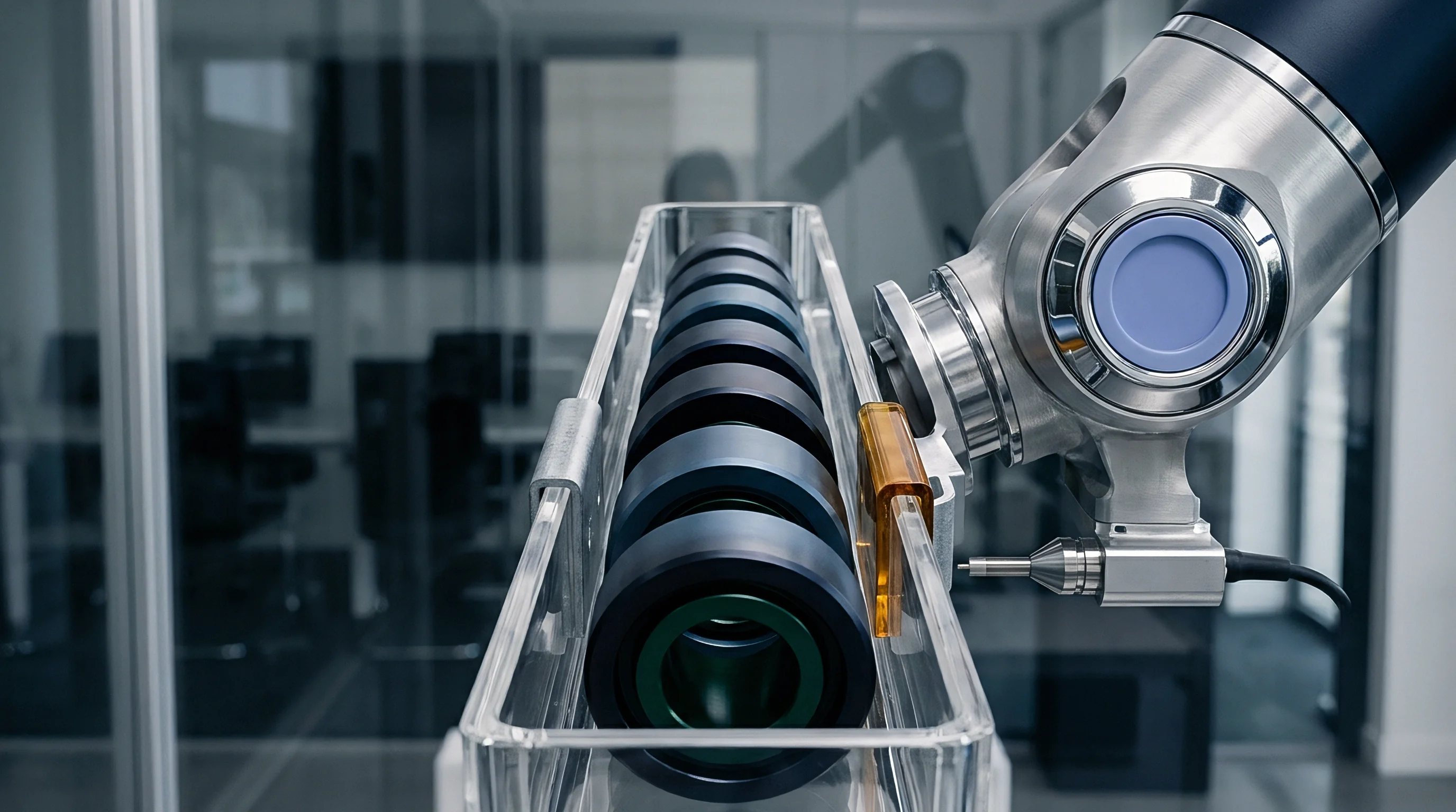
Preisach and Prandtl-Ishlinskii Operator Formulations
Continuous hysteresis loops modeled via weighted elementary relay hysterons capture rate-independent memory losses across multi-axial stress fields. The Preisach model maps environmental inputs to a continuous spectrum of bistable relay operators characterized by upper and lower switching thresholds. Weighting functions defined across the threshold plane determine the shape and saturation behavior of the resulting hysteresis curve.
Integrating Preisach operators into sensor state space models allows the tracking of minor and major environmental memory loops.
Prandtl-Ishlinskii operators utilize play and stop hysterons to provide computationally lighter mathematical structures suitable for real-time edge processing. Play operators model threshold-based backlash, while stop operators bound maximum physical displacement or saturation limits. The classical Prandtl-Ishlinskii model assumes symmetric hysteresis loops around the origin.
Environmental drift across thermal and moisture domains exhibits pronounced asymmetry due to non-symmetric material phase changes and temperature-dependent diffusion rates. Modifying the elementary play operators with generalized non-linear saturation functions corrects for asymmetric behavior across wide operating windows.
| Model Architecture | Computational Complexity | Memory Footprint | Asymmetry Handling | State Parameter Count |
|---|---|---|---|---|
| Classic Preisach Operator | High (O(N^2) per step) | Large (Threshold Grid) | Native via Density Map | 256 to 1024 Kernels |
| Generalized Prandtl-Ishlinskii | Moderate (O(N) per step) | Small (Vector Array) | Requires Non-linear Transform | 16 to 64 Weights |
| State Space Differential (Duhem) | Moderate (Matrix ODE) | Compact (State Vector) | Native via Derivative Sign | 8 to 24 Derivatives |
| Augmented Polynomial Space | Low (Static Evaluation) | Minimal (Coefficients) | Poor (Path Independent) | 10 to 30 Coefficients |
| Methods evaluated under temperature cycling between minus forty degrees Celsius and eighty-five degrees Celsius at ninety percent relative humidity. | ||||
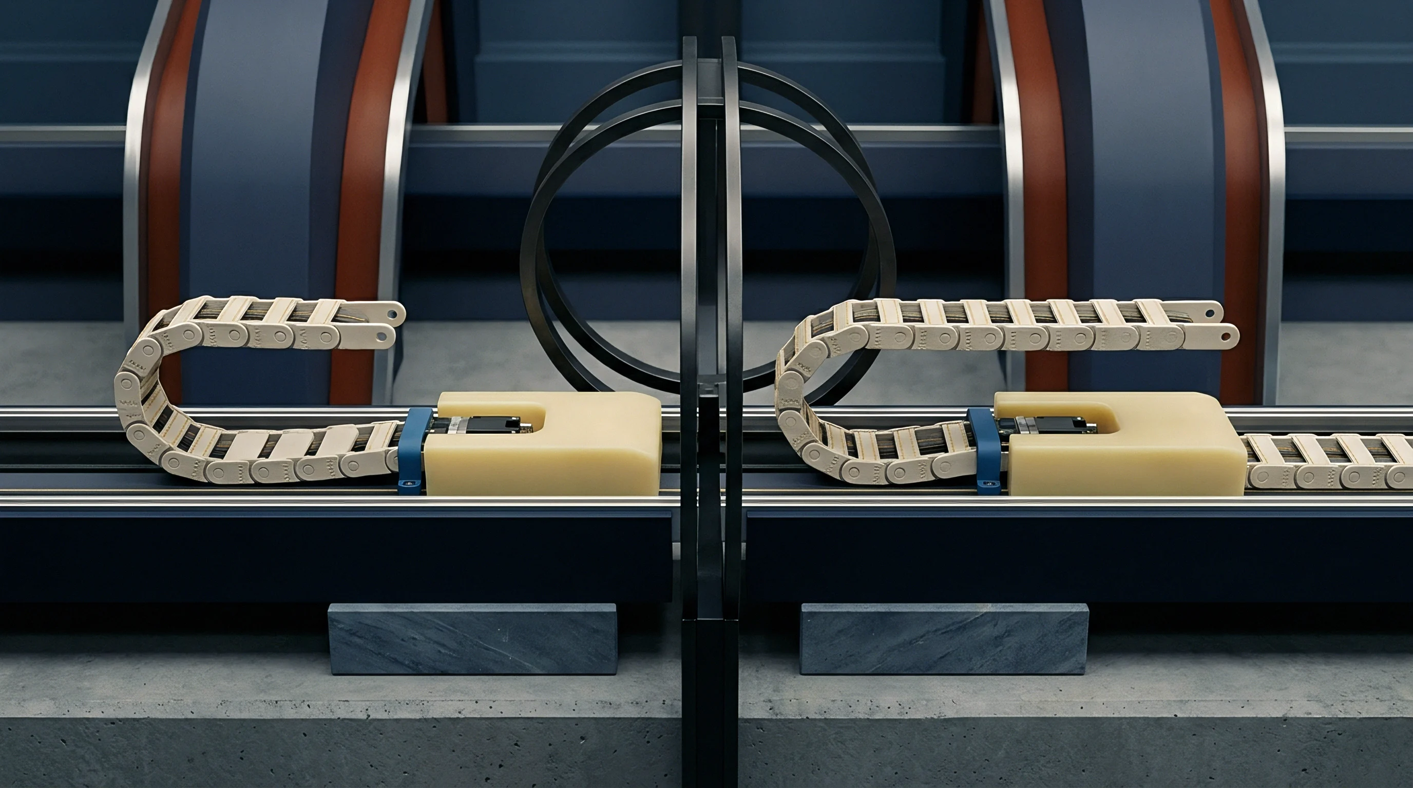
State Variable Expansion for Environmental Memory States
Incorporating history dependence into vector state equations transforms static baseline calibration equations into dynamic system representations. Standard linear state space models employ state vectors containing velocity, position, or electrical charge. Environmental state space expansion adds virtual state variables corresponding to internal material stress, absorbed moisture concentration, and thermal gradient energy storage.
Memory terms accumulate rapidly.
The state equation dictates how environmental inputs update the internal memory states over continuous time increments:
dx/dt = A(u, T) x(t) + B(u, T) du/dt + Phi(u, x_h)
The system matrix A governs the exponential decay rate of internal stress and moisture diffusion states, while input matrix B couples rate-of-change terms for temperature and strain into the state vector x(t). The vector Phi represents non-local hysteresis operators evaluated over the material memory history x_h. Static polynomials fail under cyclic loads.
By updating these internal variables at discrete sampling intervals, the state space system tracks residual die stress without storing explicit historical timestamped arrays.
A worked example demonstrates the mathematical structure of this dynamic state expansion. Consider a three-axis MEMS accelerometer subjected to thermal cycles under static one-g gravity loading. Assume an internal thermal state variable x_T representing internal package stress relaxation.
Over a thermal cycle from twenty degrees Celsius to sixty degrees Celsius and back to twenty degrees Celsius at a ramp rate of two degrees per minute, an uncompensated sensor exhibits a zero-g offset shift of eight milligals. The forward state space matrix assigns an exponential decay constant of zero point zero zero five per second to the thermal stress state. As the environmental chamber temperature increases, the internal state tracks the lag between ambient temperature and internal substrate stress.
When returning to twenty degrees Celsius, the internal state retains a value of zero point three four arbitrary stress units, corresponding exactly to the measured eight milligal zero-point offset. Subtracting the state-predicted offset from the raw voltage output restores zero-point output accuracy within zero point five milligals across the entire cycle.
Whether higher-order differential state operators can represent long-term polymer viscoelastic creep without inducing real-time matrix inversion instability remains unresolved across current metrology literature.
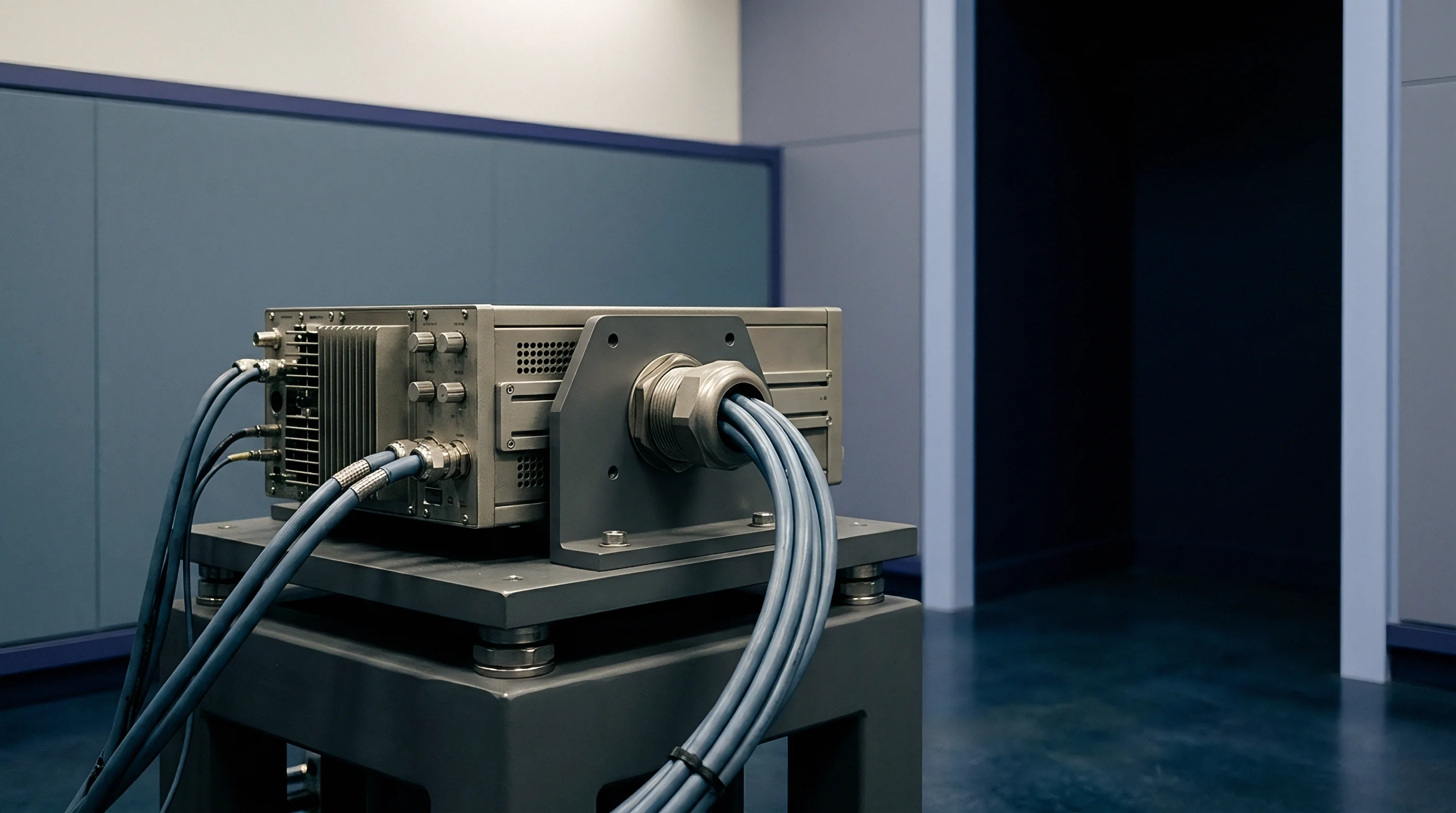
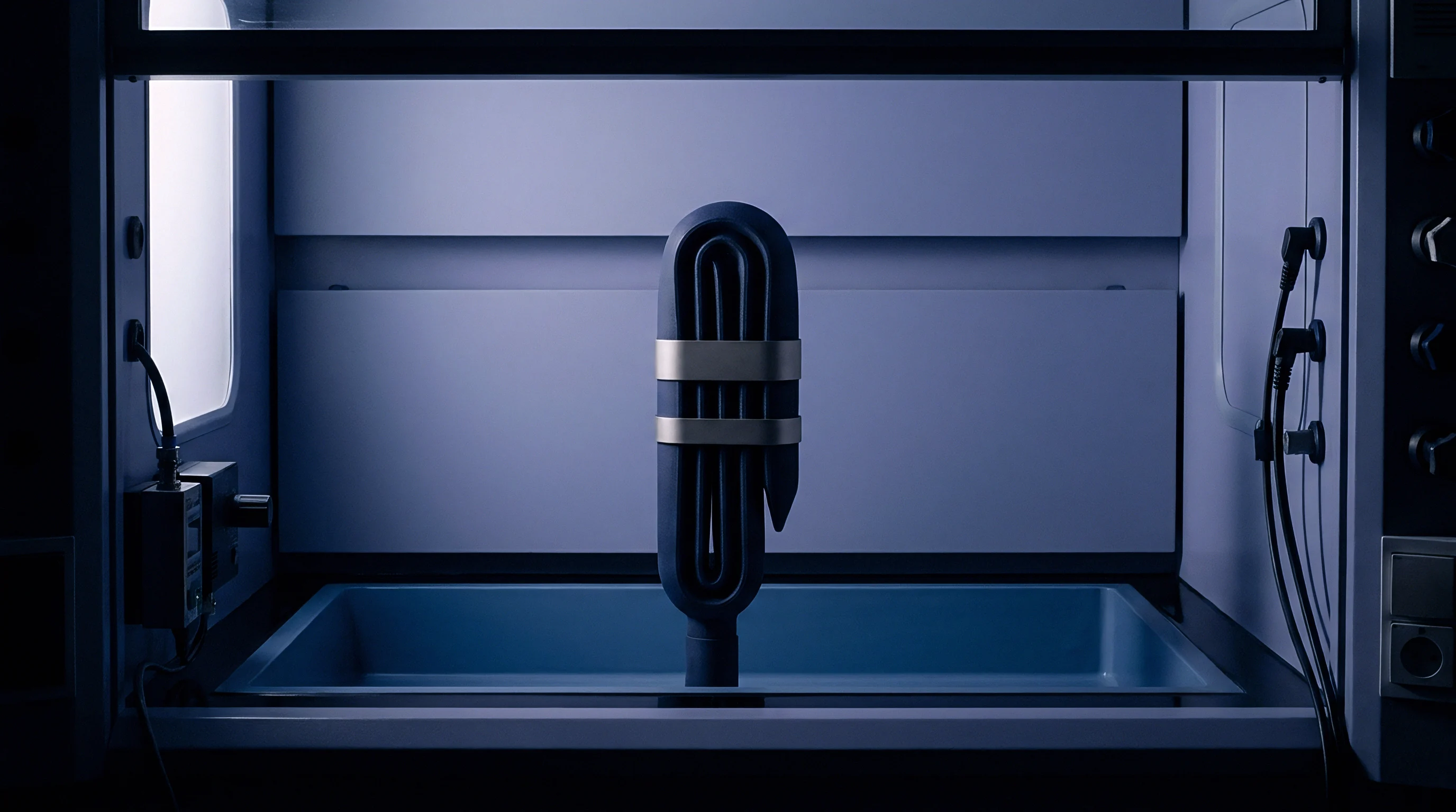
Matrix
Multivariate sensor network calibration demands real-time updating of state estimation arrays to account for cross-channel interference. In modern high-precision measurement networks, individual sensors generate raw signals that pass through digital filtering pipelines containing cross-axis coupling matrices. These calibration matrices must dynamic change their internal coefficient values when environmental conditions cross defined operational thresholds.
Static calibration matrices derived at a single factory temperature point produce significant measurement errors when deployed in unconditioned field environments.

Cross-Axis State Space Differential Equations
System matrices governing multi-axis sensor clusters capture inter-channel crosstalk through non-diagonal transfer coefficients. Primary sensitivity coefficients occupy the main diagonal of the gain matrix, while cross-axis sensitivity factors sit on off-diagonal positions. In the presence of multi-axis hysteresis, these off-diagonal terms cannot remain static constants.
They function as dynamic state variables dependent on the vector magnitude and directional path of applied mechanical loads.
Coupling matrices map raw voltage responses to true physical engineering units across multiple input channels simultaneously. Silicon die strain induces drift. The matrix transformation follows the structured continuous state space linear form:
Y(t) = C(T, RH) X(t) + D(T, RH) U(t) + E_hyst(U, X_h)
Where Y(t) is the vector of measured sensor outputs, X(t) is the expanded environmental state vector, U(t) is the physical excitation input vector, and E_hyst represents the non-linear multi-axis hysteresis vector derived from operator evaluation. Covariance matrices reflect node uncertainty. The matrix operators C and D are continuously updated via parameter maps indexed by instantaneous temperature T and relative humidity RH.
Recursive Least Squares and Unscented Kalman Filtering
Estimation algorithms inside distributed sensor nodes tracking nonlinear states maintain numerical stability during rapid ambient shifts. The Unscented Kalman Filter computes system states by propagating a deterministic set of sigma points through non-linear multi-axis hysteresis equations. Unlike Extended Kalman Filtering, which linearized non-linear functions via Jacobian matrices, the Unscented Kalman Filter preserves second-order and third-order statistical moments, accurately tracking covariance during abrupt environmental transients.
Recursive Least Squares estimation with a directional forgetting factor updates system matrices continuously when explicit non-linear models prove too computationally dense for embedded microcontrollers. The directional forgetting factor scales back historical data weighting exclusively along input channels undergoing active excitation, preserving system memory across unexcited axes.
- Covariance Matrix Conditioning prevents numerical singularity during state estimation by continuously monitoring system matrix condition numbers.
- Sigma Point Propagation projects multi-axis hysteresis uncertainty bounds through non-linear physical state updates without computing explicit Jacobians.
- Directional Forgetting Rules update active cross-coupling parameters while holding idle axis coefficients stable during single-variable environmental sweeps.
- State Vector Truncation limits internal state dimensions to essential physical memory variables, restricting real-time computation overhead.
Compliance with ISO/IEC 17025 Clause 7.8 demands that calibration certificates record full environmental history alongside expanded measurement uncertainty.
When selecting linear algebraic updating mechanisms for multi-axis sensor networks, engineering teams balance numerical accuracy against local computational constraints. Complex state matrices demand significant processing cycles, which increases local power consumption and thermal self-heating inside sealed sensor enclosures. Manufacturers routinely attribute secondary cross-channel offset shifts to unexpected PCB mounting stress rather than unmodeled state space cross-coupling dynamics.

Rig
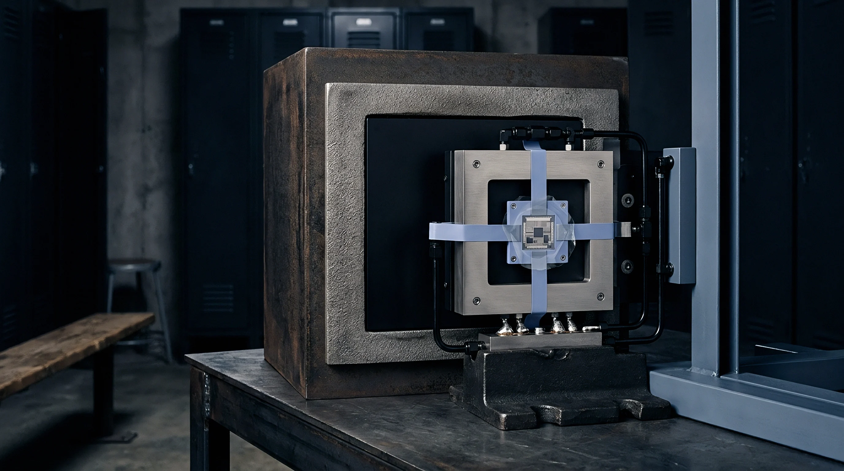
Testing high-precision transducer arrays demands climate-controlled test chambers paired with automated multi-axis mechanical actuators. Factory calibration environments must isolate the sensor under test from uncontrolled ambient vibrations, thermal fluctuations, and stray electromagnetic fields. Establishing a rigorous baseline calibration profile requires exposing the sensor network to continuous sweep profiles that systematically traverse the complete multi-dimensional operational space, including extreme boundary conditions and rate-of-change transients.
Multi-Axis Environmental Chamber Integration
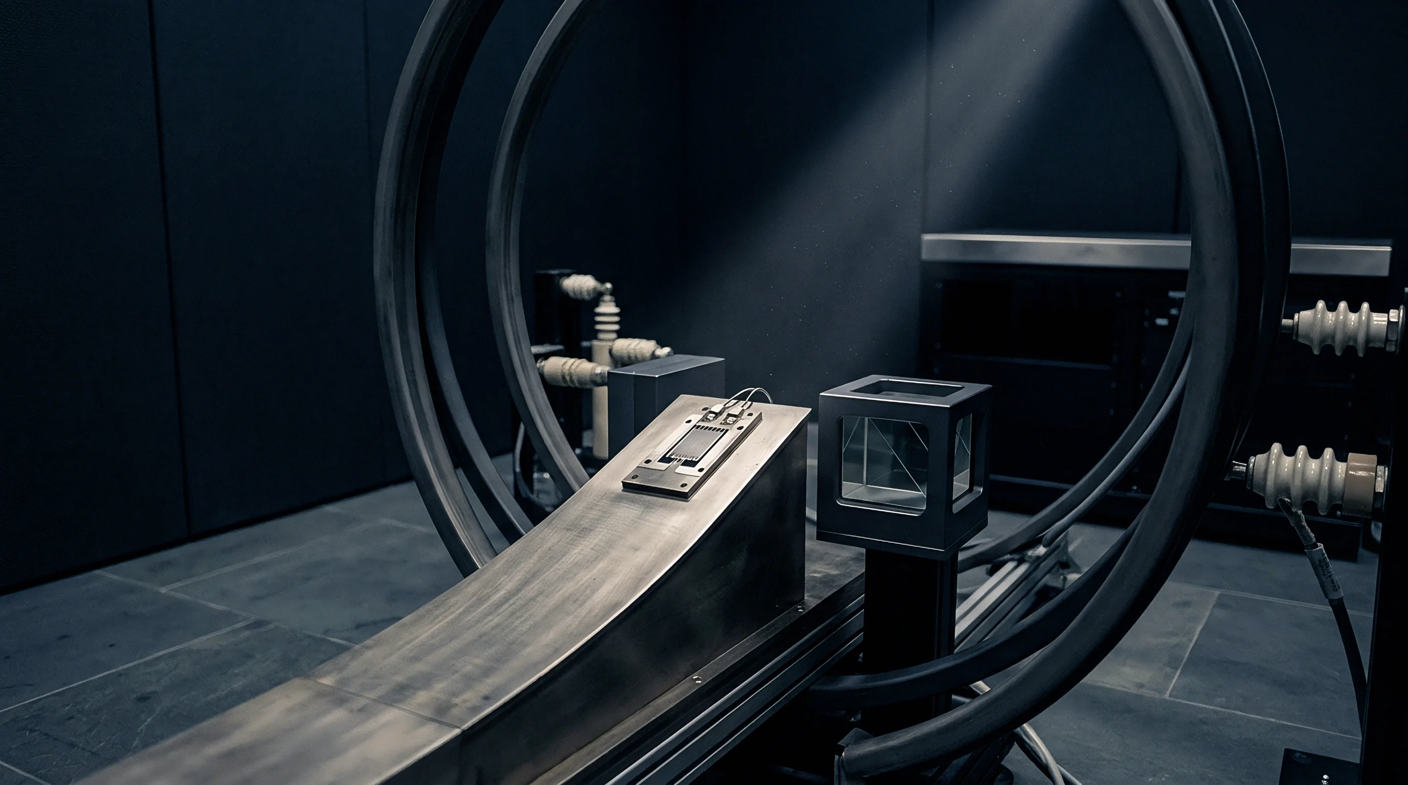
Calibrating pressure and tilt sensors under coupled thermal ramps requires synchronized nitrogen purging and multi-axis tilting tables. Standard climate chambers exhibit spatial temperature variations up to one point five degrees Celsius across the internal working volume. High-precision calibration setups utilize specialized copper equalizing blocks and forced convection ducts to limit spatial thermal gradients to within zero point zero five degrees Celsius across the target sensor array.
Relative humidity controls introduce additional testing challenges. Dew point generators must supply conditioned airflow without producing micro-condensation droplets on exposed electrical leads. Rapid humidity sweeps induce moisture concentration gradients across sensor packaging, triggering transient internal strain fields that reveal long-term viscoelastic relaxation behaviors.
Primary Standard Traceability Chains under Dynamic Loading
Reference instruments certified according to ISO/IEC 17025 establish absolute measurement confidence when ambient conditions sweep through specified ranges. Standard static calibration procedures rely on deadweight testers and primary quartz pressure reference standards maintained at reference temperatures of twenty degrees Celsius. Dynamic multi-axis environmental calibration requires reference transducers that maintain certified accuracy classes across sweeping thermal and mechanical environments.
Uncertainty budgets for dynamic environmental calibration rigs must include the reference standard uncertainty, chamber spatial non-uniformity, signal conditioning noise floors, and hysteresis model truncation residuals. Combining these uncertainty sources yields an expanded uncertainty budget governed by international metrological guidelines.
- Mount target sensor arrays onto a thermally stabilized, stress-decoupled mechanical interface plate inside the environment chamber.
- Connect reference standard transducers to parallel sampling channels located within the identical environmental zone.
- Execute a baseline dry nitrogen thermal ramp from minimum to maximum rated operating temperature at a controlled rate of zero point five degrees Celsius per minute.
- Dwell at maximum thermal limit for four hours to ensure complete material structural equilibrium and internal thermal equilibration.
- Introduce controlled humidity steps at steady-state thermal dwell points while recording continuous multi-channel output voltages.
- Apply multi-axis mechanical excitations using calibrated automated tilt actuators or force application pistons across each thermal and humidity step.
- Log raw multi-channel voltage, reference standard outputs, internal temperature sensor readings, and exact sampling timestamps to a centralized data engine.
Thermal stabilization times double for every additional millimeter of stainless steel housing thickness surrounding an uncompensated sensor die.
Calibration rigs must maintain mechanical integrity throughout extended thermal cycling routines. Structural thermal expansion within the mounting rig itself can introduce parasitic mechanical loads onto the sensor housing, contaminating cross-axis hysteresis measurements. A test chamber never changes ambient temperature faster than the thermal mass of the reference sensor can achieve uniform internal thermal equilibrium.

Algorithm
Field compensation routines execute digital filtering strategies that inverse-model memory-dependent sensor distortions in real time. Embedded firmware installed inside modern sensor network nodes processes raw analog-to-digital converter counts through integrated digital signal processing blocks. These digital blocks run matrix multiplication routines and hysteretic operator evaluations to generate fully compensated physical engineering output values.
Efficient algorithm design minimizes computational latency and memory consumption, enabling high sampling rates on low-power microcontrollers.

Real-Time Matrix Inversion and Memory Kernels
Embedded digital signal processors update non-linear compensation coefficients using truncated history lookup windows. Direct dynamic matrix inversion demands significant computing resources, scaling with the cube of the state vector dimension. To circumvent matrix inversion latency during embedded operation, field algorithms utilize pre-calculated inverse hysteresis operators or feedforward neural network approximations optimized during factory calibration passes.
Truncated lookups reduce computing overhead. The inverse Prandtl-Ishlinskii operator provides an analytical closed-form solution for hysteresis compensation. If a forward hysteresis model uses play operators with specific threshold density distributions, an inverse operator structure with identical mathematical form can be analytically constructed by transforming the threshold parameters and density weights.
Evaluating the inverse operator requires only basic arithmetic operations, vector dot products, and simple threshold conditional checks, making it suitable for low-power microcontroller deployment.
| Algorithmic Strategy | Residual Error (% FSO) | Execution Latency (us) | SRAM Usage (KB) | Flash Memory (KB) |
|---|---|---|---|---|
| Static 3rd Order Polynomial | 0.450 | 12 | 0.5 | 4.0 |
| Inverse Prandtl-Ishlinskii (16 Play) | 0.035 | 85 | 2.1 | 12.5 |
| State Space Kalman Filter (8 States) | 0.015 | 340 | 8.4 | 48.0 |
| Direct Preisach Grid Inversion | 0.008 | 1450 | 64.0 | 256.0 |

Networked Cross-Calibration Node Propagation
Distributed sensor nodes share covariance values across digital buses to refine individual compensation coefficients without central controller overhead. In large-scale sensor networks monitoring industrial process plants or aerospace structures, individual nodes experience varying micro-environmental conditions. Nodes equipped with highly accurate, low-drift reference sensors can broadcast their environmental state estimates and local measurement variances over controller area network buses or wireless mesh protocols.
Adjacent sensor nodes consume these broadcast states to execute cross-calibration routines. If a secondary node detects a drift in its internal temperature or strain reading that deviates from the local spatial consensus, it updates its internal state space covariance matrix. Matrix inversion dominates processor latency.
The node auto-adjusts its off-diagonal state coupling coefficients to compensate for regional environmental gradients without requiring removal from active field service.
A worked example details the networked auto-calibration sequence. Consider a industrial pipeline monitoring node measuring differential pressure under external ambient thermal swings. The node contains a local piezoresistive sensor and receives wireless ambient temperature updates from two neighboring structural monitoring nodes.
Over a twelve-hour operating window, the local node records an uncompensated baseline pressure shift of zero point one eight bar due to solar heating. The local node executes a state space update using an eight-state Kalman filter. The state vector incorporates local pressure, local die temperature, broadcast ambient temperature from neighbor nodes, and local die-attach strain state.
Processing the state update step reduces output uncertainty from zero point one eight bar down to zero point zero one two bar. System execution latency remains below two hundred microseconds per sample interval, consuming less than ten kilobytes of system RAM.
Evaluating state vector consistency across distributed nodes prevents localized sensor failures from corrupting global network calibrations. Uncompensated hysteresis destroys zero stability. Algorithms running inside field nodes must flag anomalously large state variance jumps, isolating degraded sensor hardware before erroneous data propagates upstream into primary control loops.
Invoking section six point four of ISO/IEC 17025 shifts the verification threshold from static factory calibration certificates to dynamic continuous recalibration logs.

Exposure
Uncertainty growth over extended operational lifetimes generates measurable commercial liabilities through warranty claims and out-of-tolerance sensor outputs. Sensor manufacturing practices often prioritize initial factory accuracy figures listed on marketing datasheets over long-term field stability metrics. A high-precision transducer rated for zero point zero one percent full scale accuracy at twenty degrees Celsius can drift to zero point five percent full scale after twelve months of continuous field exposure to thermal cycles and ambient moisture ingress.
This drift creates significant financial exposure for system integrators operating under tight end-product performance guarantees.
Yield Losses and Field Recalibration Intervals
Inaccurate zero-point drift predictions inflate factory rejection rates while shortening acceptable operational windows between service checks. When manufacturing plants perform single-point factory testing, sensors with high internal residual stresses pass initial quality control checks. Once deployed, these units experience rapid stress relaxation and moisture absorption, drifting out of specification within weeks.
Incorporating multi-axis hysteresis screening during factory testing increases initial scrap rates by five to fifteen percent but eliminates early-life field returns.
Field recalibration costs exceed initial purchase. Recalibrating high-precision sensor networks in industrial facilities demands specialized mobile calibration carts, certified reference standards, and trained service technicians. Extending recalibration intervals from twelve months to thirty-six months dramatically lowers total lifecycle operating expenditures for end users.
- Factory Scrap Rate Inflation occurs when multi-axis thermal dynamic testing screens out units exhibiting unacceptably high internal die stress.
- Warranty Return Liabilities scale directly with unmodeled long-term viscoelastic creep in sensor bonding adhesives.
- Mobile Field Recalibration Costs include labor, vehicle dispatch, reference standard hire, and operational plant downtime during verification procedures.
- Tiered Unit Pricing Structures allow manufacturers to sell compensated, low-drift sensor units at a three-fold price premium over basic uncompensated transducers.
Uncompensated cross-axis hysteresis generates cumulative state tracking errors that compound over successive environmental cycles.

Contractual Tolerance Limits and Rejection Criteria
Procurement specifications specifying total uncorrected sensor drift dictate unit pricing structures and warranty liabilities. Buyers specifying sensor networks for critical defense, aerospace, or semiconductor manufacturing infrastructure must write explicit environmental hysteresis test conditions into primary procurement contracts. These clauses must define maximum allowable drift limits under dynamic thermal ramps, specified relative humidity ranges, and combined multi-axis strain cycling.
Contractual rejection criteria must mandate that suppliers provide full state space model parameters and certified uncertainty budgets alongside physical hardware deliveries. Relying on simple static calibration certificates transfers the financial risk of long-term environmental drift entirely onto the buyer. This residual uncertainty directly determines whether a sensor array maintains its target specification class or drops into a lower performance tier after twenty-four months of field service.