Calibration Interval Optimization for Industrial Temperature Transducers
Optimizing calibration intervals balances in situ sensor drift history against consumer risk to minimize total plant ownership costs without violating tolerances.

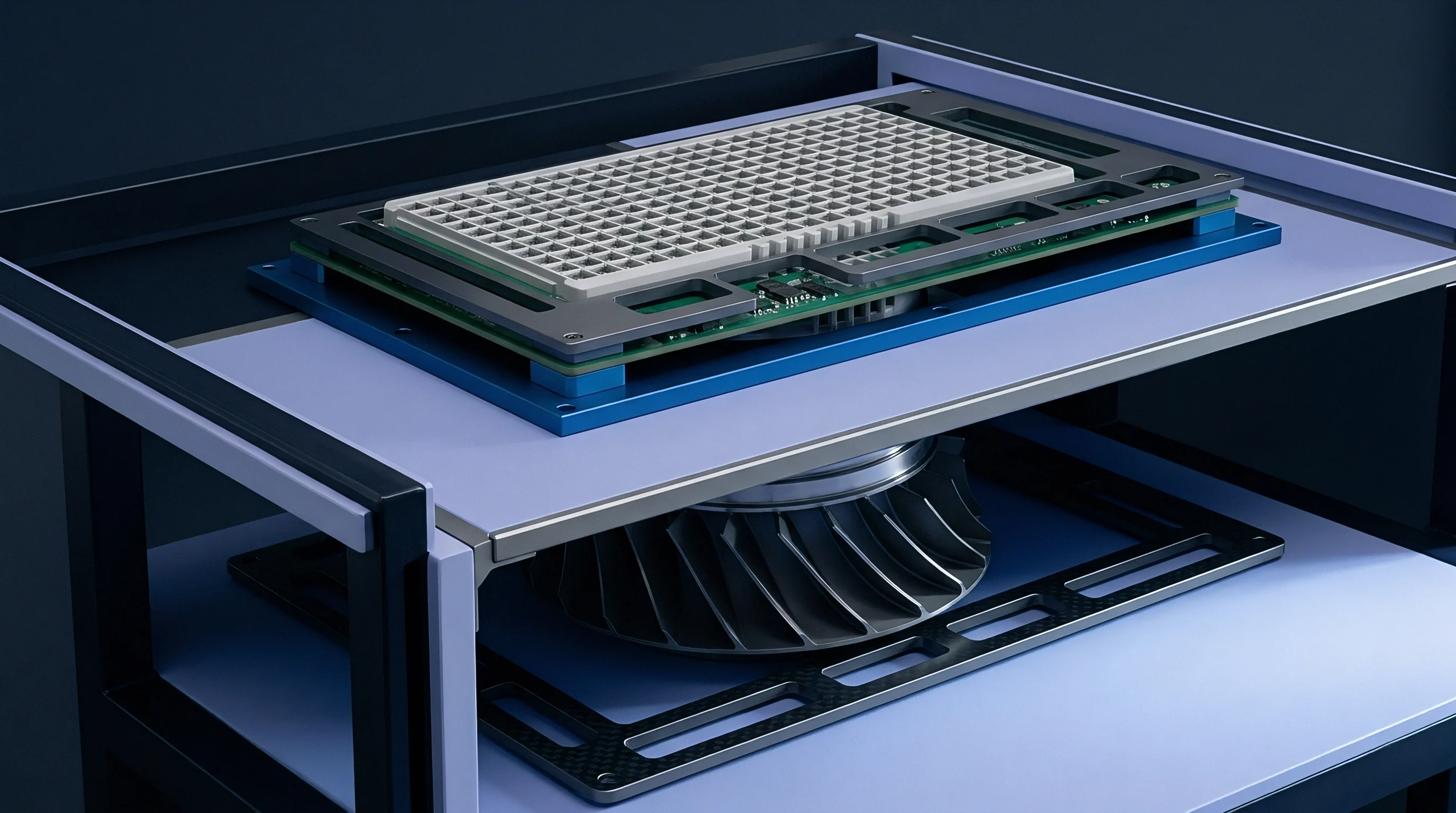
Sheath
An unannealed mineral-insulated Pt100 sensor held at 420 degrees Celsius drifts 0.38 Kelvin within its initial two hundred hours of continuous operation. Factory calibration certificates issued at room temperature mask this early movement entirely. Industrial temperature transducers, whether platinum resistance thermometers or base-metal thermocouples, depend on mechanical packaging that degrades under combined thermal, vibrational, and chemical exposure.
Optimization of recalibration intervals begins with the physical rate of sensor degradation rather than calendar conventions.
Platinum elements anneal under heat. When thin-film or wire-wound resistance detectors operate at elevated process levels, internal residual stresses from manufacturing relax. This metallurgical settling creates a predictable zero-point offset before long-term drift mechanisms take command.
Conversely, thermocouples undergo preferential oxidation of alloy legs, fundamentally altering the Seebeck coefficient along thermal gradients across the sheath length.
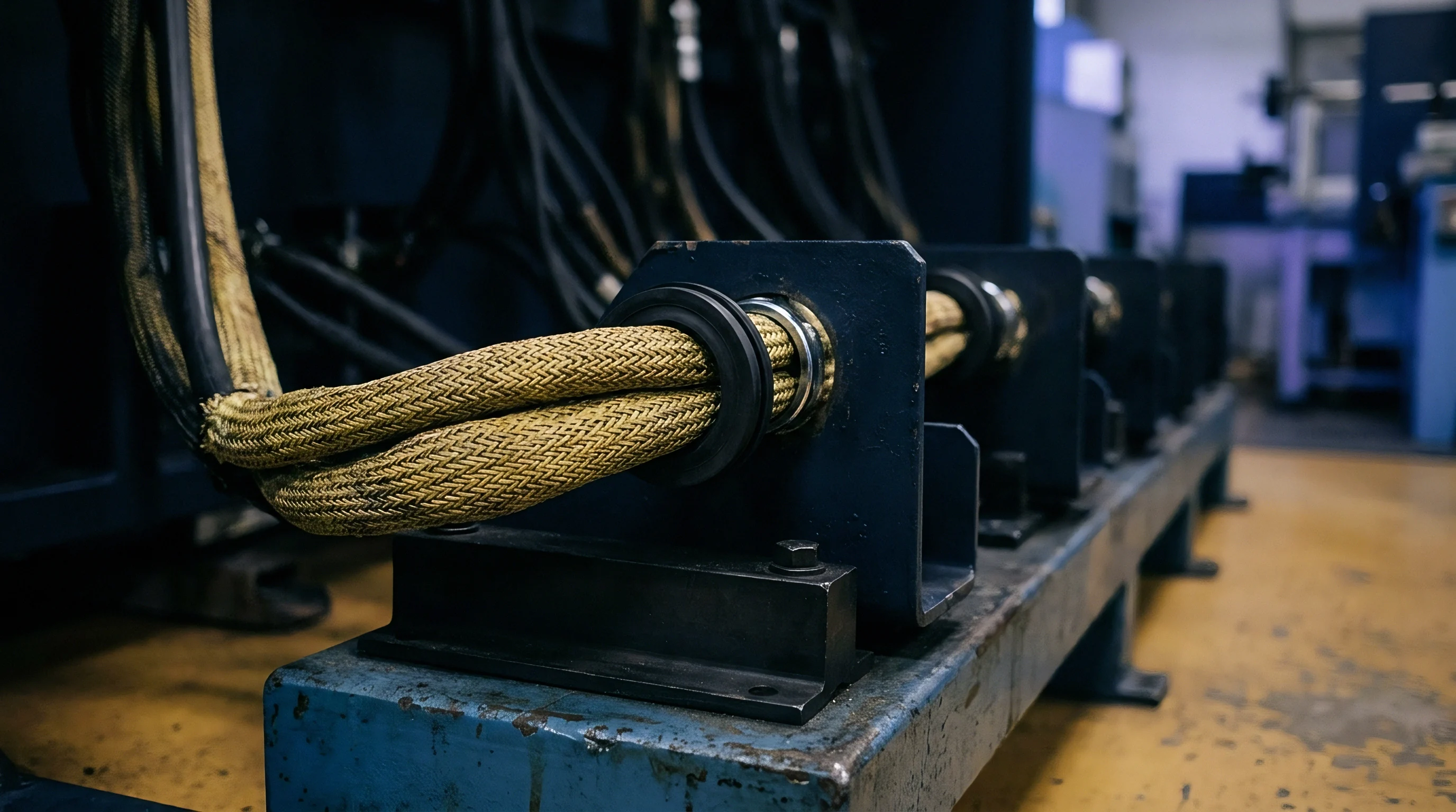
Thermal Shunting and Insulation Resistance
Direct current leakage through packed magnesium oxide powder degrades signal integrity when operating temperatures exceed 500 degrees Celsius. Ceramic insulation resistance drops exponentially with rising heat, establishing parallel parasitic electrical paths across the sensing loop. For a 100-ohm RTD, an insulation degradation down to 100 kilohms induces a negative measurement error of approximately 0.25 Kelvin at process conditions.
Cold junctions introduce ambient offsets. Ice points disclose offset errors. Standard loop transmitters cannot isolate this shunting error from true process changes during standard operations.
Standard IEC 60751 specifies that insulation resistance below 100 megohms at 500 degrees Celsius invalidates sensor conformity.
Moisture ingress through compromised terminal seals creates similar shunting problems at lower operational temperatures. Mineral insulation absorbs atmospheric moisture rapidly when protective potting seals crack during thermal cycling. This contamination produces erratic, non-linear resistance swings that periodic single-point bench tests often fail to diagnose if the bench environment lacks process humidity.
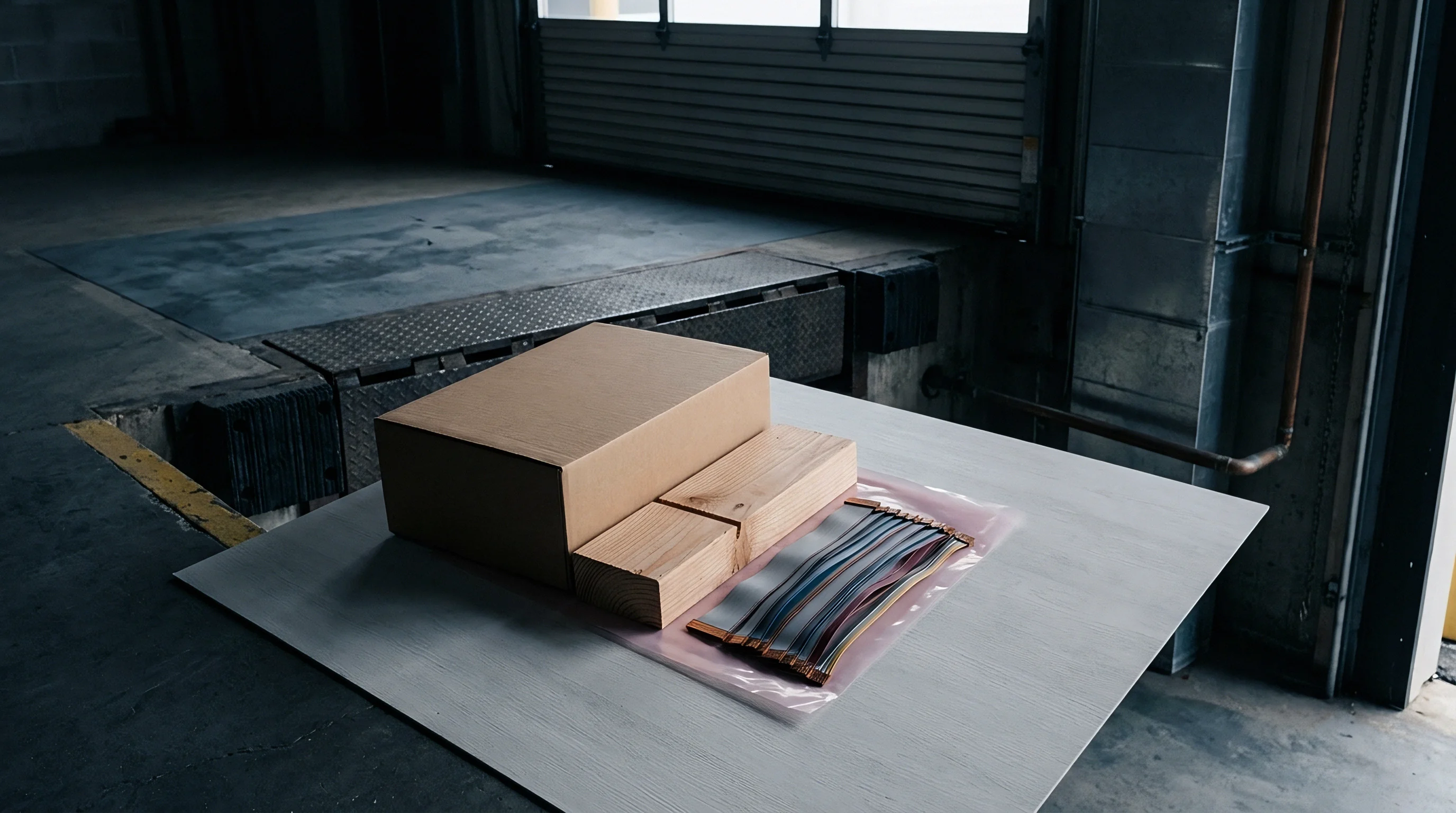
Mechanical Stress and Grain Boundary Slip
Vibrational acceleration across process pipework induces lattice defects in thin-film resistance tracks. Sensor housings transmit structural vibration directly to unsupported internal lead wires, causing work hardening and micro-fractures. In aggressive chemical environments, atmospheric contaminants diffuse through protective metal sheaths over prolonged service campaigns.
- Green rot attack affects nickel-chromium thermocouple conductors exposed to marginally oxidizing atmospheres between 800 and 1050 degrees Celsius, destroying thermoelectric calibration.
- Platinum grain growth weakens sensor resistance windings under continuous high-temperature exposure, accelerating calibration offset shifts.
- Insulation moisture absorption degrades shunting resistance across lead wires, driving negative measurement offsets in humid plants.
- Lead wire work hardening results from pipework vibration and induces intermittent open circuits during operational cycles.
High temperatures accelerate metallurgical changes. Process vibration breaks internal welds. Undetected thermal drift across uninspected temperature elements leads directly to bulk chemical batch contamination and forced product disposal.
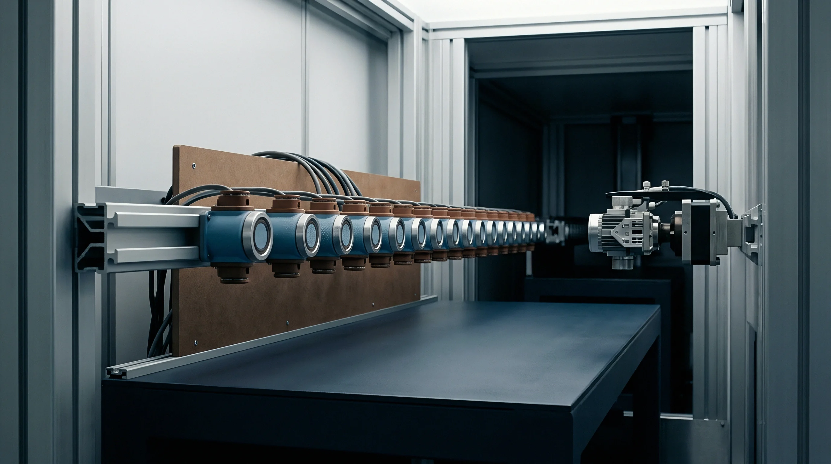
Tolerance
Guard banding definitions dictate whether an instrument remains fit for thermal control loops. Evaluating an industrial sensor requires separating process tolerance limits from measurement capability. When a plant specifies an operating window of plus or minus 1.0 Kelvin, allocating that entire margin to sensor drift invites compliance failure.
Metrological uncertainty introduced by dry-wells, reference probes, and digital readouts consumes a substantial portion of the nominal process tolerance band.
Process transmitters contribute electronic span drift. Digital convertor circuits shift with seasonal cabinet temperatures, adding errors onto the primary element drift. Calculating realistic recalibration intervals requires modeling these combined error sources as a single measurement loop.
A class A thin-film platinum resistor held at 500 degrees Celsius for 1,000 hours shows a typical positive drift of 0.42 Kelvin.

Test Uncertainty Ratios and Consumer Risk
Accredited dry-well calibrators introduce measurement variance that alters the statistical probability of false acceptance. Standard metrology rules recommend maintaining a Test Uncertainty Ratio of four to one between process tolerance and calibration system uncertainty. Where calibration systems operate with a two to one ratio, false accept risk increases markedly, allowing drifting sensors to pass verification checks while operating outside process specifications.
| Transducer Type | Temperature Band | Annual Drift (k=2) | Calibration Uncertainty | Maximum TUR |
|---|---|---|---|---|
| Pt100 Class A Thin-Film | -50 to 200 °C | ±0.15 K | ±0.05 K | 3.0:1 |
| Pt100 Class A Wire-Wound | 200 to 450 °C | ±0.35 K | ±0.08 K | 4.4:1 |
| Type N Thermocouple (Class 1) | 400 to 900 °C | ±1.20 K | ±0.45 K | 2.7:1 |
| Type K Thermocouple (Class 1) | 400 to 1100 °C | ±2.80 K | ±0.60 K | 1.7:1 |
False reject risks introduce equal commercial waste by forcing premature replacements of conforming hardware. When calibration guard bands are set too conservatively to eliminate false accept risk, conforming sensors near the margin face unnecessary disposal. Calibrating intervals around statistical drift patterns preserves production yields without degrading safety tolerances.

Does in Situ Degradation Exceed Operating Limits?
Process transmitters subjected to ambient temperature swings display analog-to-digital conversion errors separate from the primary sensing tip. Industrial installations frequently expose field-mounted electronics to summer ambient peaks reaching 55 degrees Celsius followed by sub-zero winter exposures. These ambient fluctuations produce temperature coefficient drift within the transmitter ranging from 0.005 to 0.015 Kelvin per degree of ambient shift.
Thermocouple extension cables add cold-junction compensation errors. Mineral-insulated cables routed through hot process zones generate secondary thermal voltages along compositional inhomogeneities. Systematic drift demands span adjustments.
Shorter intervals suppress plant risk. Suppliers routinely argue that published drift specifications apply solely to pristine laboratory test conditions rather than industrial thermowells.
Model
Document OIML D 10 structures mathematical methods for evaluating whether calibration frequencies match physical drift rates. Preserving fixed calendar intervals across diverse manufacturing units introduces systematic inefficiencies. Stable measurement loops undergo excessive testing, while sensors placed in punishing environments wander out of tolerance months before scheduled recalibration.
Moving from rigid schedules to data-driven intervals relies on statistical tracking of historical as-found data.
Interval management relies on formal adjustment algorithms. Simple staircase methods step inspection windows outward or inward based on pass or fail results from consecutive test events. Advanced control chart methods track individual drift vectors to forecast the exact operational month when cumulative drift crosses established guard bands.
Statistical Drift and Interval Adjustment
Observed calibration offsets plotted across consecutive inspection cycles reveal whether sensor degradation follows linear aging or random shock distributions. Platinum elements under moderate operating conditions exhibit predictable square-root-of-time aging drift. This structural predictability permits mathematical modeling of interval extensions using historical calibration records.
Higher operating temperatures accelerate sensor drift and demand shorter calibration intervals.
The OIML D 10 document outlines five primary methods for adjusting calibration intervals across industrial instrument fleets:
- Automatic staircase adjustment extends the operating interval by a predetermined percentage upon a conforming test result and contracts the interval instantly upon an out-of-tolerance finding.
- Control chart tracking plots drift magnitude against elapsed operating hours to extrapolate the date when measurement error reaches acceptable limits.
- Calendar time grouping clusters similar temperature probes across plant zones and shortens the interval for the entire group if a target percentage fails.
- In-service operating hours logging decouples calibration timing from calendar dates by triggering verifications through plant DCS runtime counters.
- In situ comparative cross-checking identifies outlier drift continuously by comparing redundant sensor pairs within the same thermowell assembly.
| Method Classification | Data Prerequisite | Extension Factor | Contraction Factor | Operational Risk |
|---|---|---|---|---|
| Staircase Method | Consecutive single tests | +10% to +15% | -25% to -50% | Moderate |
| Control Chart Method | Minimum 5 calibration cycles | Linear extrapolation | Immediate pull | Low |
| Homogeneous Fleet Grouping | Fleet population data (>30 units) | Statistical 95% pass rate | -20% across fleet | Moderate |
| Runtime Hour Logging | DCS runtime telemetry | Proportional to base hours | Proportional to hours | Low |
Response Criteria across Variable Service Windows
Operating hours inside hostile media produce wear rates that calendar-based scheduling fails to track. A reactor temperature sensor cycling daily between ambient and 400 degrees Celsius experiences structural fatigue faster than an identical sensor monitoring a steady-state storage tank. Logging operational hours and thermal excursions via distributed control systems creates the quantitative dataset needed for dynamic interval calculation.
Pure alumina insulators resist shunting. Clause 7.1 of OIML D 10 permits interval extension only when historical in-tolerance probability exceeds ninety-five percent across consecutive test cycles.
Audit
Historical inspection dossiers provide the empirical baseline for extending or contracting recalibration dates. Quality departments frequently archive calibration certificates as passive compliance artifacts without mining the numeric delta between as-found and as-left states. Calculating drift velocity requires extracting this numerical difference and normalizing it against elapsed service time.
As-found data exposes undetected drift. The as-found measurement records the true condition of the transducer prior to any zero adjustments or span trimmings. When a technician trims an instrument without logging the initial deviation, the operational history necessary to justify interval optimization is destroyed.
Thermocouple decalibration remains invisible to external electronics until secondary reference probes enter the process thermowell.
Historical in Situ Verification Data
Portable dry-block comparators deployed directly on running process lines capture drift without extracting the probe assembly. Extracting deeply seated mineral-insulated probes from thermowells risks cold-working internal wires and creating artificial shifts that were absent during process operation. In situ comparison against calibrated secondary reference standards eliminates handling artifacts from calibration datasets.
Robust historical dossiers track several physical parameters across every inspection cycle:
- As-found deviation values quantify raw drift from the preceding operating cycle at defined calibration setpoints.
- Operating environment parameters capture thermal cycling counts, ambient temperature ranges, and exposure to corrosive vapors.
- Transmitter configuration data record damping factors, analog trim values, and reference junction temperature readings.
- Reference standard traceability documents calibration certificates and expanded measurement uncertainty values for checking equipment.
Historical calibration records govern intervals. Systematic analysis of these inspection dossiers reveals whether drift rates accelerate over sensor lifespan. Many thin-film sensors show minimal movement during their initial year, followed by rapid non-linear drift once protective ceramic coatings degrade.
Are Fixed Calendar Cycles Metrologically Defensible?
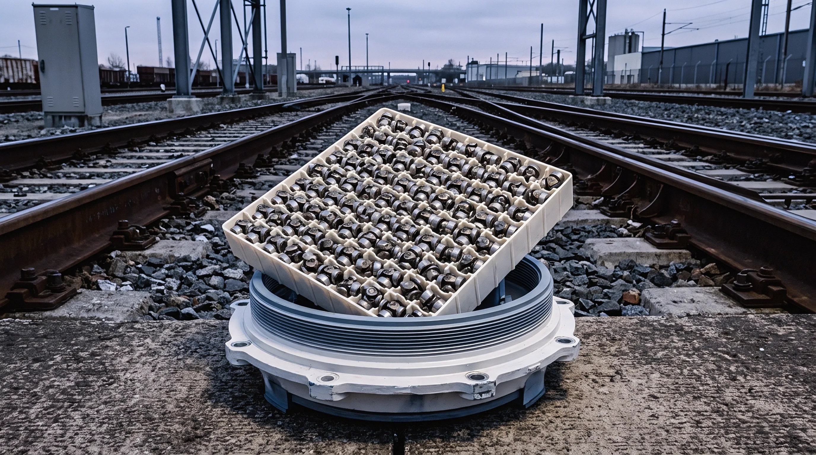
Preset twelve-month inspection cadences remain standard practice across industrial chemical facilities. These arbitrary intervals originate in administrative accounting schedules rather than transducer physics. A thermocouple operating continuously near its metallurgical limit degrades within three months, while an RTD in clean thermal oil remains within Class A limits for five years.
Engineers still dispute whether automated drift algorithms can accurately differentiate between pure sensor aging and sensor contamination without physical extraction from the thermowell.

Ledger
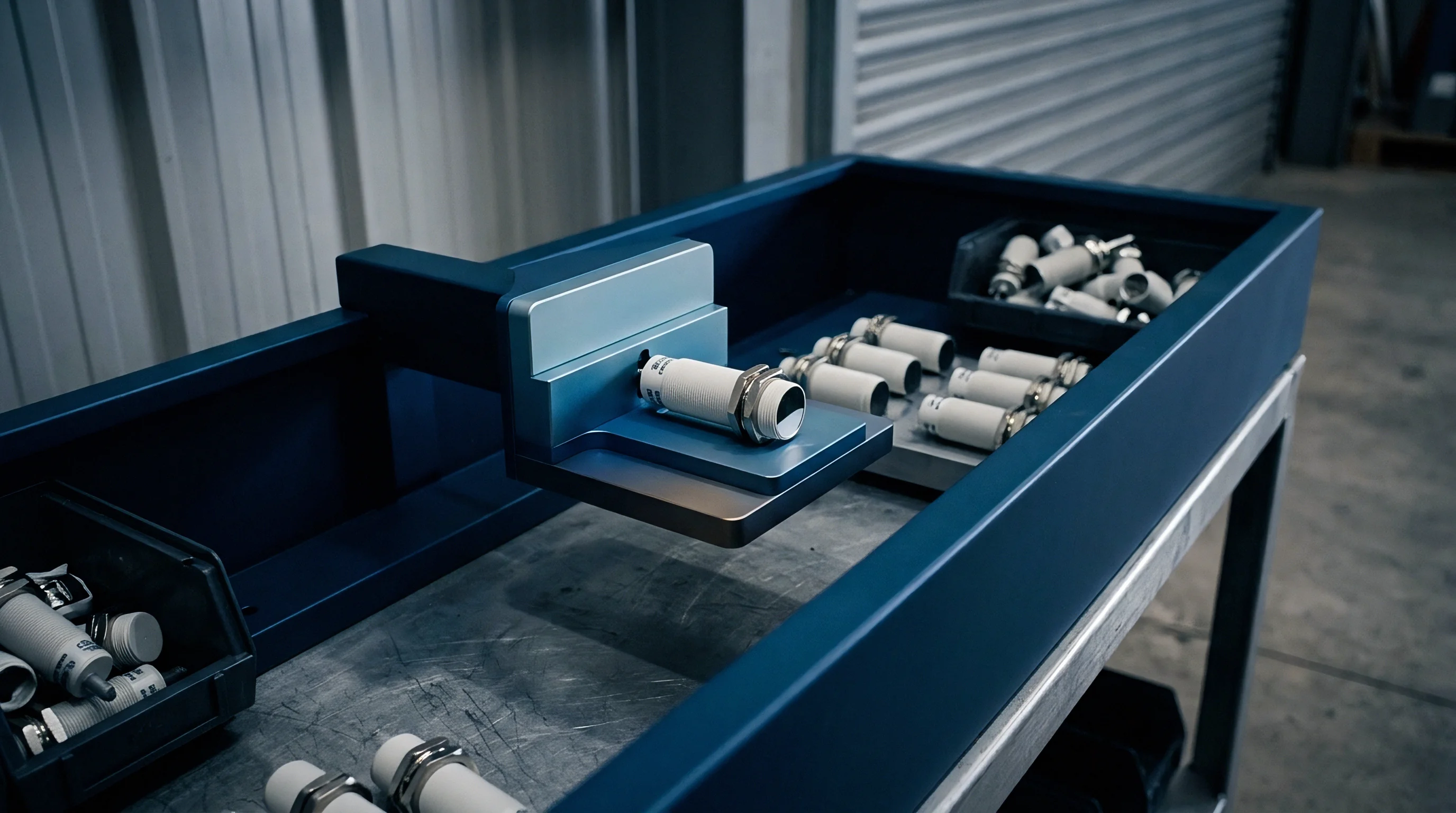
Direct laboratory invoices form only a fraction of total thermal measurement operating expenses. Pulling an operational sensor involves mechanical permits, line isolations, transmitter un-wiring, and temporary process shutdowns. The landed cost of a twenty-minute bench verification frequently exceeds the purchase price of the primary transducer when labor overhead enters the calculation.
Periodic recalibration consumes maintenance budgets. Unscheduled downtime carries steep penalties. Extending an interval from twelve to twenty-four months across a plant housing two thousand temperature transmitters halves recurring calibration labor while preserving line uptime.
Lifecycle Expenditure and Calibration Frequency
Plant technicians spend substantial labor hours pulling assemblies from active thermowells, packing them for shipping, and restoring seals. When calibration management systems double inspection intervals on stable non-critical points, internal labor shifts to managing severe thermal wear points. This resource reallocation improves overall plant measurement reliability while lowering net operational expenditure.
| Calibration Strategy | Interval Length | Annual Pulls | Calibration Labor | Out-of-Spec Risk |
|---|---|---|---|---|
| Fixed Calendar Base | 12 Months | 500 | $87,500 | Medium |
| Arbitrary Stretch | 24 Months | 250 | $43,750 | High |
| OIML D 10 Dynamic Model | 6 to 36 Months | 215 | $37,625 | Very Low |
| In Situ Verification Routine | 18 Months (In Situ) | 110 | $24,200 | Low |
| Cost figures reflect average loaded technician rates of $70 per hour and standard laboratory verification fees. | ||||

Balance between False Acceptance and Servicing Costs
Lengthening recalibration intervals reduces third-party testing fees while heightening out-of-spec product quarantine liabilities. An optimized calibration program sets inspection schedules at the point where the cost of further interval contraction equals the statistical risk cost of production contamination. Rigorous quantitative tracking of transducer drift rates replaces guesswork with defensible metrological balance.
Process measurement intervals belong at half the duration observed to produce tolerance excursions during normal operation.