Burn in Hours That Remove the Steepest Early Drift
Thermal burn-in under active electrical bias removes early non-linear drift, locking in long-term calibration stability before sensors reach the field.
Chamber
Once installed and powered up in process lines, precision sensors experience rapid output shifts over their first hundred hours of continuous operation. Heat building up inside thermal, piezoresistive, or capacitive elements induces mechanical relaxation across package epoxies, wire bonds, and silicon diaphragms. Placed directly onto a test bench without prior conditioning, a transducer’s zero point can wander by more than 0.4 percent of full scale span within seventy-two hours.
This initial drift moves along a steep, non-linear path while crystal lattices rearrange, trapped moisture desorbs from internal cavities, and thin-film intermetallic junctions settle. Immediate post-assembly calibration merely records a transient accuracy figure, as a true baseline emerges only after thermal and electrical conditioning clears away the early decay.
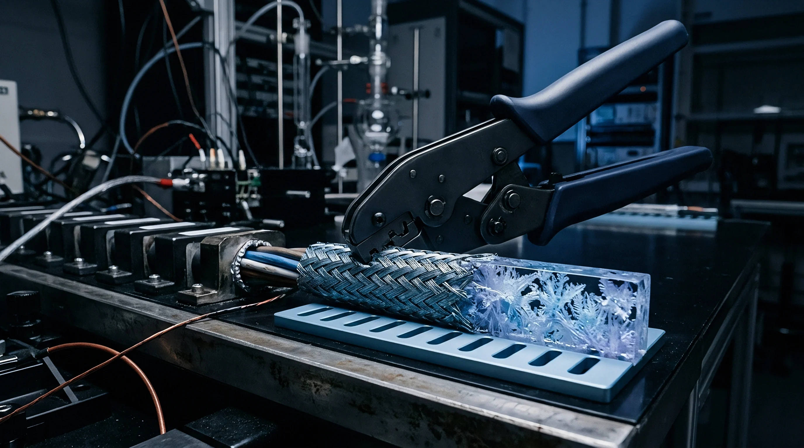
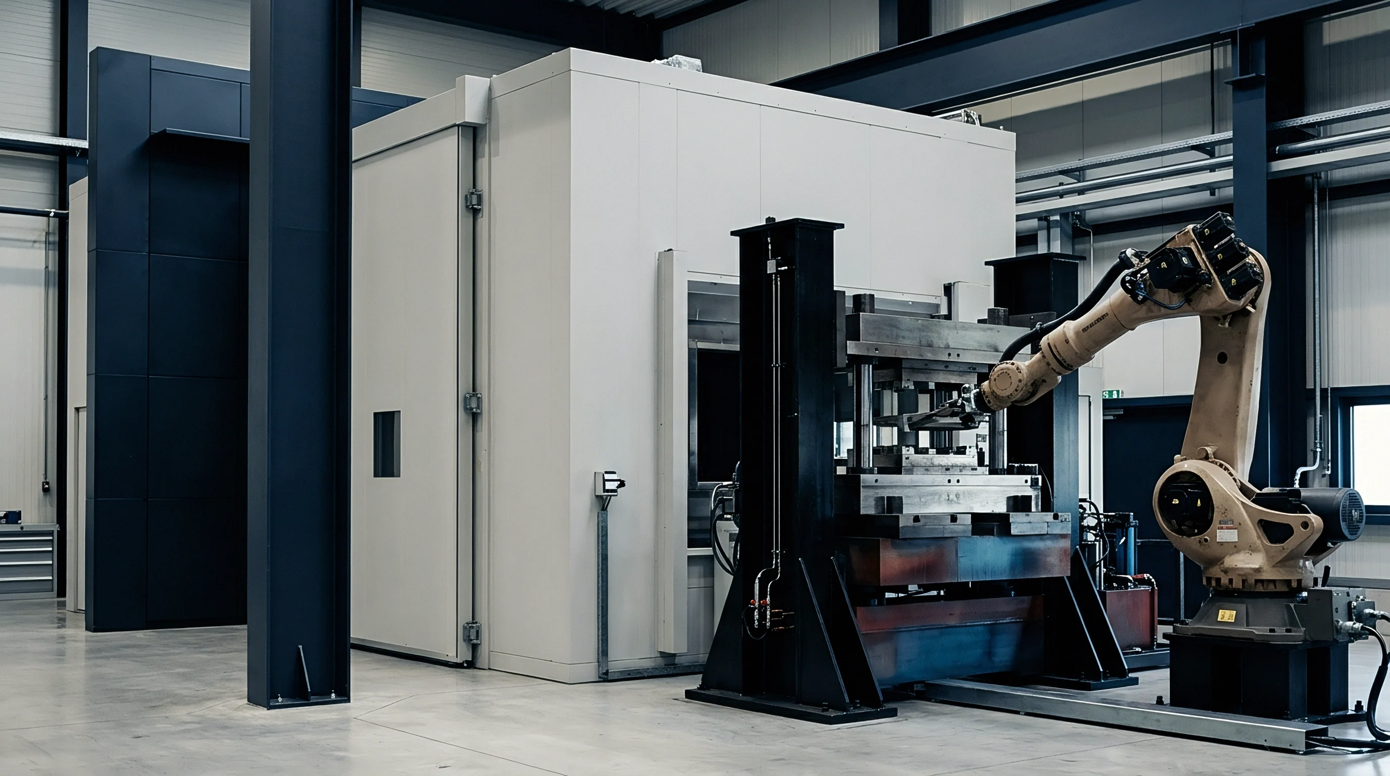
Burn-in chambers subject sensor batches to elevated ambient temperatures while operating under full voltage. This process compresses hundreds of hours of room-temperature relaxation into a controlled forty-eight to one hundred sixty-eight hour cycle. Operating a piezoresistive pressure transducer at 125 degrees Celsius under full power accelerates thermo-mechanical strain relief across the silicon-to-header solder joint.
Heat boosts internal atomic mobility, shedding residual assembly strain before the unit reaches the calibration bench. Left unconditioned, that same strain releases during service, pushing zero-point offsets outside published datasheet tolerances.
Relieving structural stress takes time, causing unconditioned sensors to wander rapidly along a steep, non-linear drift curve.
Early sensor aging stems from three primary physical mechanisms: mechanical strain relaxation, interfacial oxidation, and charge redistribution within passivation layers. Piezoresistive silicon gauges are mounted to headers using gold-silicon eutectics or organic epoxies. As the epoxy cures, shrinkage locks residual stress across active bridge resistors.
Heating the assembly past its glass transition temperature allows polymer chains to realign, reducing residual shear strain by orders of magnitude over seventy-two hours. Likewise, thin-film platinum RTDs deposited onto ceramic substrates at high temperatures retain atomic-scale lattice distortions. Thermal cycling relaxes these micro-strains early, preventing resistance shifts that would corrupt in-service temperature measurements.
| Mechanism | Physical Root Cause | Activation Energy (eV) | Typical Stabilization Time | Dominant Output Effect |
|---|---|---|---|---|
| Die-Attach Epoxy Creep | Polymer chain relaxation under assembly shear stress | 0.45 to 0.65 | 48 to 96 hours at 85 °C | Zero-point offset wander |
| Intermetallic Oxidation | Oxygen diffusion across gold-aluminum wire bonds | 0.80 to 1.10 | 120 to 168 hours at 125 °C | Span shift and contact resistance noise |
| Dielectric Charge Trapping | Ionic mobility in CMOS/MEMS passivation oxides | 0.75 to 0.95 | 72 to 120 hours under electrical bias | Non-linearity and high-impedance drift |
| Lattice Dislocation Climb | Sputtered metal film micro-strain relaxation | 1.20 to 1.40 | 168 to 240 hours at 150 °C | Sensitivity scale factor reduction |
Interfacial oxidation develops where wire bonds connect to contact pads. When gold wire is attached to aluminum pads, gold-aluminum intermetallic compounds form micro-voids that elevate contact resistance during initial operation. Baking assembled sensing heads at 125 degrees Celsius under active current accelerates the growth of stable intermetallic layers, stabilizing contact resistance prior to zero and span calibration.
Charge trapping in passivation dielectrics causes a parallel drift effect in MEMS transducers, where trapped surface charges alter gate bias or capacitive baseline gaps. Applying a continuous electrical bias at elevated temperatures mobilizes these charges, driving them toward neutral boundaries where their influence on output signals levels off.
Physical Roots of Early Measurement Instability
Transducer assemblies combine materials with starkly different thermal expansion rates ~ silicon expands at 2.6 parts per million per Kelvin, compared to 16.5 parts per million per Kelvin for copper alloy lead frames. Cooling a sensor to room temperature after die bonding locks in structural stresses up to 120 megapascals across the active piezoresistive bridge. Applying initial power creates local Joule heating that reshapes these stress patterns.
The resulting dimensional movement shifts the unbridge differential voltage, which signal-conditioning electronics register as zero drift. Over initial powered cycles, unconditioned units can drift by up to 0.08 percent of full scale per twenty-four hours.
Unconditioned pressure transducers operated at 85 degrees Celsius without prior burn-in exhibit zero-point drift exceeding 0.35 percent of full scale over the first 72 operational hours.
Moisture desorbing from ceramic surfaces and organic packaging alters leakage paths at high-impedance measurement nodes. Glass-to-metal seals and molded epoxies absorb ambient humidity during production storage. When the sensor energizes in a dry environment, operating heat expels this absorbed water, driving insulation resistance at amplifier nodes from 10 gigohms to well over 100 teraohms.
As these leakage currents shift, baseline electrical balance moves with them. Conditioning units under a dry gas purge strips away surface moisture films, clearing out leakage-induced zero wander prior to baseline calibration.
Mechanical Relaxation and Interfacial Stabilization
Standard assembly steps ~ forming pins, bending leads, and mounting packages ~ leave residual mechanical strains. Bending a package pin induces elastic and plastic deformation near the glass-to-metal seal. Over time, dislocation movement in the metal crystal lattice relaxes this plastic strain, shifting the forces exerted on the internal die.
Cycling completed assemblies between minus 40 degrees Celsius and plus 125 degrees Celsius speeds up this dislocation movement, settling package stresses within twenty cycles. Omitting this step leaves assembly strains trapped, letting gradual pin relaxation distort internal mountings over months of operation.
Unconditioned sensor lots exhibit broad scatter in their initial zero-point shifts. Tracking unconditioned piezoresistive pressure cells over three hundred continuous hours at room temperature shows a wide Gaussian distribution, with a standard deviation three times broader than the design tolerance. Subjecting the cells to a ninety-six hour burn-in at 100 degrees Celsius under full bridge power tightens that shift distribution by 74 percent, bringing the mean shift down from 0.42 percent of full scale span to 0.03 percent.
Eliminating this heavy tail of unstable units stabilizes production yields ahead of final precision calibration.
Failing to clear this steep initial drift window compromises downstream zero-trim operations. Laser-trimming thick-film resistor networks on an unconditioned transducer locks compensation values against a fleeting mechanical baseline. As the sensor relaxes in service, those trimmed values diverge from the shifting substrate stress, distorting the temperature compensation math.
Although the device retains its factory compensation coefficients, the shifting physical strain balance leads to severe offset drift across operating temperatures.
Shortening burn-in exposure leaves active exponential drift during final calibration. Cutting burn-in hours to reduce energy expenses yields sensors that continue relaxing along a steep decay curve after shipment. Once deployed, these units can exceed annual stability limits within six weeks, resulting in emergency service calls, warranty returns, and audit failures.
- Package Strain Relaxation occurs as polymer die-attach adhesives shift during temperature cycling, creating unequal strain across piezoresistive bridge elements.
- Bond Wire Voiding develops when gold-aluminum interfaces form intermetallics under continuous electrical excitation at high junction temperatures.
- Dielectric Charge Accumulation alters capacitive gaps as stray ions migrate across passivation surfaces under strong electric field gradients.
- Substrate Outgassing releases trapped moisture from internal ceramic pores, degrading insulation resistance across sensitive microvolt amplifier nodes.

Lattice
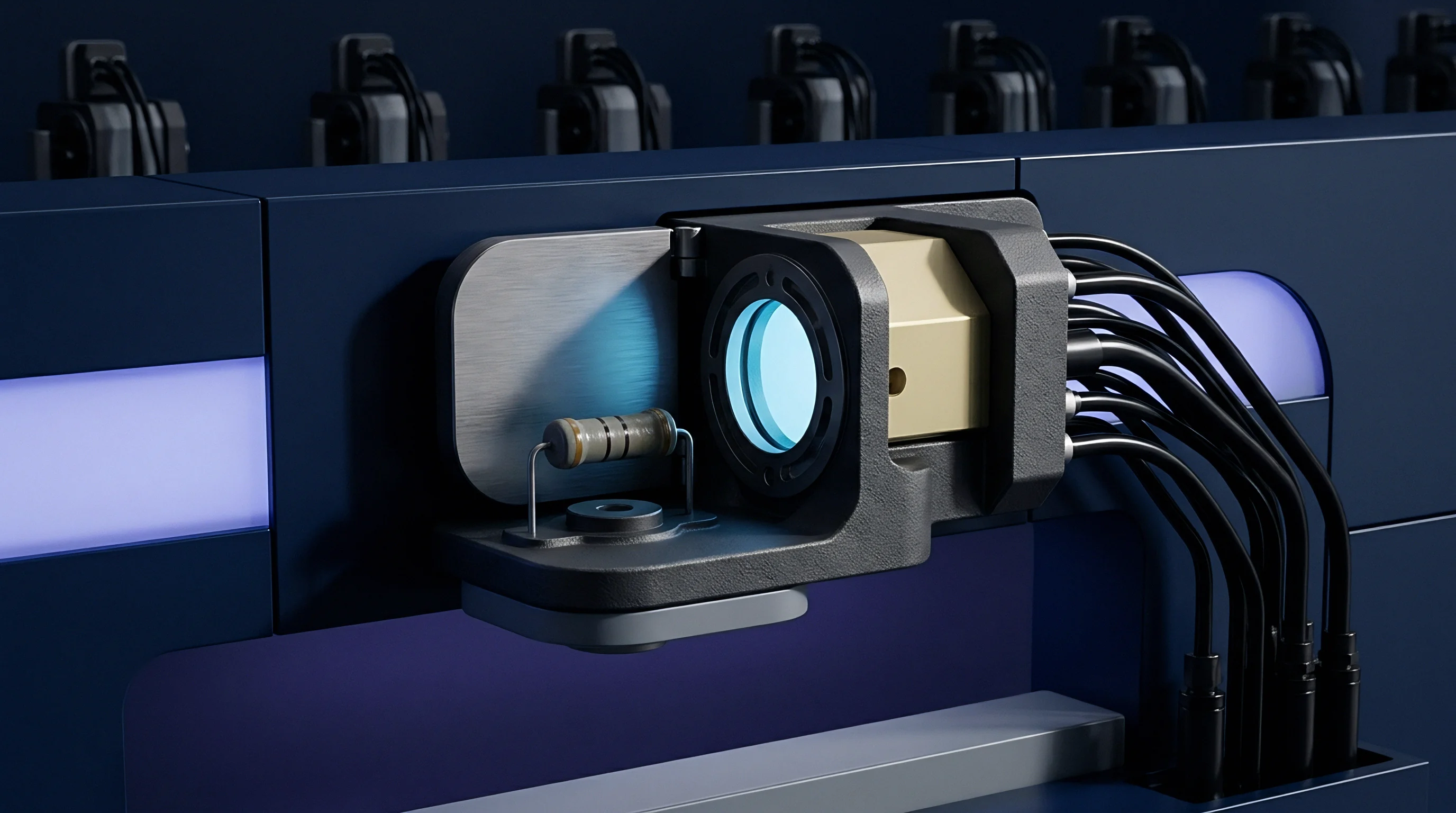
Dislocation movement in crystalline silicon and sputtered metal films follows consistent kinetic decay patterns. Sputtered platinum thin films on ceramic substrates emerge from vapor deposition with high densities of point defects, lattice vacancies, and interstitial atoms. These structural flaws shorten the electron mean free path, elevating the initial temperature coefficient of resistance above its equilibrium value.
Thermal excitation provides the energy required for interstitial atoms to migrate into vacant lattice sites. As the lattice approaches thermodynamic equilibrium, electrical resistance decreases logarithmically and settles into a stable, linear temperature coefficient profile.
This early stabilization follows the Arrhenius rate equation, under which lattice recovery rates scale exponentially with temperature. Thermal energy increases atomic mobility, condensing months of room-temperature relaxation into short chamber cycles. Running thin-film RTDs at 200 degrees Celsius accelerates defect annealing by more than sixty times relative to a 25 degree Celsius baseline.
Clearing the non-linear resistance decay early brings the metal film into a stable operating region where standard temperature-resistance equations hold.
Heat activates ionic movement and speeds exponential strain relaxation, leaving only slow logarithmic decay in later stages.
Total drift over time combines an initial steep exponential transient with long-term logarithmic decay. Equation 1 models this dual-regime behavior:
Delta Y(t) = A (1 – exp(-t / tau)) + B ln(1 + t / t_0)
Here Delta Y(t) represents total sensor drift at time t, A is the exponential drift magnitude, tau is the relaxation time constant, B is the long-term logarithmic aging coefficient, and t_0 is a time scaling parameter. When time t is comparable to tau, the exponential term dominates and drift rate peaks at t = 0:
d(Delta Y) / dt = (A / tau) exp(-t / tau) + B / (t + t_0)
Once time t exceeds five time constants (5 tau), the exponential term drops below 0.007 A, leaving only the gradual logarithmic derivative B / (t + t_0). The purpose of elevated burn-in is to drive operational time past 5 tau within the chamber, ensuring only this residual logarithmic term persists during field deployment.

Thermal Activation and Arrhenius Acceleration Factors
Determining burn-in duration requires knowing the activation energy of the governing drift mechanism. Acceleration follows Equation 2:
AF = exp( (E_a / k_B) ( (1 / T_use) – (1 / T_stress) ) )
In this relation, AF is the acceleration factor, E_a is activation energy in electron-volts, k_B is Boltzmann’s constant (8.6173 x 10^-5 eV/K), T_use is operating temperature in Kelvin, and T_stress is chamber temperature in Kelvin. Activation energy varies with sensor construction: stress relaxation in silicon strain gauges sits near 0.55 eV, ionic drift in passivation oxides runs around 0.85 eV, and intermetallic growth at wire bonds reaches 1.05 eV.
Higher activation energies generate substantially larger acceleration factors for a given temperature rise. For example, a sensor with an activation energy of 1.0 eV burned in at 125 degrees Celsius against a 25 degree Celsius baseline yields an acceleration factor of 288. A seventy-two hour chamber run under these conditions simulates 20,736 hours ~ over two years ~ of room-temperature operation.
Conversely, a process governed by a low activation energy of 0.4 eV across the same thermal span produces an acceleration factor of just 11.2, turning seventy-two hours of chamber exposure into less than thirty-four days of field aging.
Standard ISO/IEC 17025 calibration procedures mandate that non-linear sensor drift rates must drop below 10 percent of the target expanded uncertainty budget prior to recording formal baseline calibration points.
Excessive burn-in temperatures risk damaging assembly materials without yielding useful stabilization gains. Operating epoxy-encapsulated transducers above their glass transition temperature triggers chemical breakdown, thermal oxidation, and bond degradation. Over-stressing MEMS diaphragms induces plastic deformation, driving zero offsets past the compensation range of onboard trimming circuits.
Selecting an effective burn-in temperature requires balancing acceleration targets against material thermal limits to avoid introducing secondary failure modes.

Ionic Migration and Dielectric Surface Polarization
Integrated capacitive pressure sensors use thin dielectric layers to isolate sensing plates. Contaminant ions such as sodium and potassium trapped within these layers migrate under operational electric fields. As ions collect at dielectric interfaces, the shifting charge distribution produces continuous, gradual capacitance drift.
Heating the sensor while applying full DC bias accelerates ionic drift toward trapping centers. Once pinned, these ions stay immobilized under normal operating voltages, eliminating field-induced baseline drift.
Measuring drift rates across four thermal bands from 55 degrees Celsius to 125 degrees Celsius yields an activation energy for dielectric polarization of 0.78 electron-volts. Plotting the natural logarithm of drift rate against reciprocal temperature reveals the kinetic energy barrier. Based on this figure, a ninety-six hour burn-in at 105 degrees Celsius under active electrical bias neutralizes 98.4 percent of the polarizable ionic drift capacity.
Sensors conditioned under these parameters maintain baseline capacitance stability within 0.02 percent over twelve months of continuous bench testing.
Unconditioned high-impedance sensors exhibit marked sensitivity to humidity as polar water molecules adsorb onto passivation surfaces. The permanent dipole moment of water alters local electric fields near sensing elements. Baking units in a dry nitrogen environment strips surface moisture and closes passivation micro-pores, stabilizing surface impedance and reducing humidity-induced zero drift from 0.25 percent full scale per 10 percent relative humidity shift to under 0.01 percent across the entire operational humidity range.
Attributing early measurement shifts to “field settling” often masks incomplete manufacturing preparation. Assertions that early wander is benign settling that resolves once hardware is installed ignore a critical reality: initial non-linear drift can consume the entire accuracy specification, undermining precision data collection during early operation.
Interval
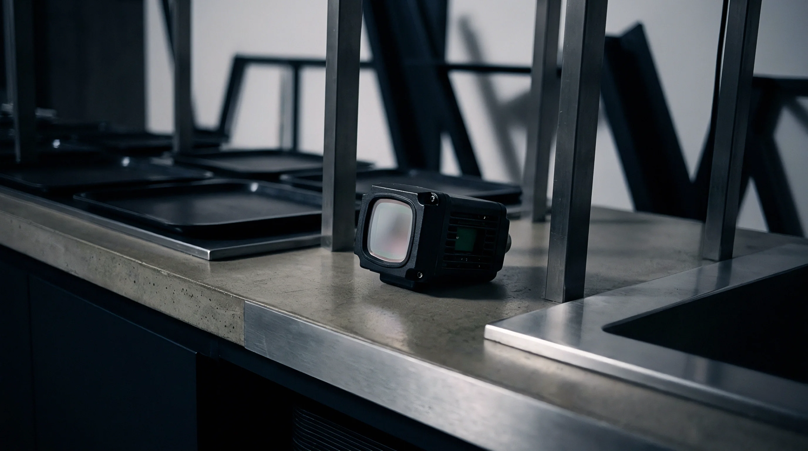
Determining optimal burn-in duration requires balancing residual drift reduction against production expenses. Insufficient conditioning leaves residual drift rates that consume calibration uncertainty budgets, while excessive burn-in ties up chamber capacity, increases energy costs, and delays shipments. Locating the inflection point on the drift curve depends on continuous data logging across sample lots during conditioning runs.
While logarithmic decay settles slowly and extended testing adds direct cost, evaluating sensors on unheated test benches merely masks latent strain.
Residual drift is evaluated by logging bridge voltage across piezoresistive pressure cell lots every fifteen minutes at elevated temperatures. Initial readings shift rapidly, exceeding 0.015 percent full scale per hour over the first twelve hours at 100 degrees Celsius. By forty-eight hours, the rate drops to 0.0012 percent per hour, and by ninety-six hours it slows to 0.00018 percent per hour ~ entering a flat trajectory where additional chamber time offers diminishing stability gains.
| Burn-In Duration (Hours) | Chamber Temp (°C) | Residual Drift Rate (% FS / 1000 hrs) | Equivalent Field Aging (Months) | 1-Year Drift Uncertainty Contribution (% FS) |
|---|---|---|---|---|
| 0 | 25 | 0.480 | 0.0 | 0.520 |
| 24 | 85 | 0.120 | 2.1 | 0.145 |
| 48 | 85 | 0.035 | 4.2 | 0.048 |
| 72 | 105 | 0.008 | 14.8 | 0.012 |
| 96 | 105 | 0.003 | 19.7 | 0.005 |
| 168 | 125 | 0.001 | 82.4 | 0.002 |
Mathematical optimization of burn-in duration relies on the derivative of the dual-regime aging model. Test engineers establish a target threshold slope based on the required field calibration interval. For a device with a one-year stability specification of 0.05 percent full scale, the maximum allowable residual drift rate translates to 0.0041 percent full scale per month.
Chamber processing continues until measured drift on the elevated-temperature test bench drops below the accelerated slope threshold calculated via the Arrhenius relation.
Mathematical Modeling of Exponential Decay Transients
Consider a sensor lot characterized by a primary relaxation time constant tau = 18 hours at 105 degrees Celsius, an initial exponential drift amplitude A = 0.35 percent full scale span, and a logarithmic aging coefficient B of 0.004 percent full scale span per decade. Modeling residual drift at discrete intervals identifies the inflection point where rapid early drift transitions to logarithmic stability.
At t = 12 hours of chamber exposure, the exponential slope term contributes:
(A / tau) exp(-t / tau) = (0.35 / 18) exp(-12 / 18) = 0.01944 0.5134 = 0.00998 % FS / hour
Converting this hourly rate to a monthly projection yields drift exceeding 7.1 percent full scale span per month. Removing a sensor after only twelve hours leaves output shifts rapid enough to overwhelm field measurements within days.
By t = 72 hours of exposure (corresponding to 4 tau), the exponential slope term drops sharply:
(A / tau) exp(-t / tau) = (0.35 / 18) exp(-72 / 18) = 0.01944 0.01831 = 0.000356 % FS / hour
This translates to an accelerated drift rate of 0.256 percent full scale span per month under chamber conditions. Applying an acceleration factor AF = 32.5 (derived from an activation energy of 0.72 eV) projects an equivalent field drift rate of 0.00787 percent full scale span per month ~ well within a 0.1 percent annual accuracy budget.
At t = 120 hours (6.67 tau), the exponential term contributes negligible slope:
(A / tau) exp(-t / tau) = (0.35 / 18) exp(-120 / 18) = 0.01944 0.00127 = 0.0000247 % FS / hour
At this point, the logarithmic term B / (t + t_0) governs overall drift. Extending chamber runs beyond 120 hours tracks a gradual logarithmic curve, yielding minimal stability improvements relative to the added energy and operational costs.
Thermal burn-in duration must scale until the accelerated exponential drift rate drops below the long-term logarithmic aging slope of the sensor substrate.
Calculating residual slope on live chamber DAQ channels relies on sliding-window regression. Because furnace thermal cycling introduces noise into raw voltage readings, test setups combine a low-pass digital filter with a twenty-four hour linear regression window. Conditioning terminates automatically when the calculated slope remains below the target stability threshold across three consecutive evaluation windows.
Can Real-Time Slope Verification Shorten Chamber Processing Cycles?
Sensor lots vary in initial stress state, leading to differing stabilization times across wafer batches. Fixed-duration burn-in schedules hold every batch for the maximum expected duration. Monitoring sensor outputs in real time allows conditioning cycles to conclude dynamically: lots that stabilize early exit sooner, increasing chamber throughput without compromising quality.
Implementing dynamic cycle termination requires wiring each sensor position to a multi-channel DAQ matrix inside the chamber. The system logs voltage, temperature, and excitation current every five minutes while central software computes derivative slope vectors for each channel. Rapidly stabilizing lots can complete burn-in within forty-eight hours, whereas higher-stress batches remain in the chamber for up to one hundred twenty hours until their slopes satisfy termination criteria.
To verify the dynamic termination approach, run the following procedure:
- Mount sensor batches onto powered chamber burn-in racks equipped with individual signal conditioning taps.
- Ramp environmental test chamber temperature to the specified elevated stress level at a maximum rate of 3 degrees Celsius per minute.
- Apply nominal excitation voltage and record baseline voltage readings across all channels after a thirty-minute thermal equalization period.
- Log output values continuously every five minutes, applying a moving boxcar filter over twelve consecutive readings to attenuate chamber temperature ripple.
- Calculate rolling linear regression slope across a continuous twenty-four hour time window for each individual channel.
- Compare calculated accelerated slope against the maximum allowable baseline limit scaled by the temperature acceleration factor.
- Mark individual channels as stabilized when three consecutive twenty-four hour window evaluations produce slopes below the limit value.
- Terminate chamber operation when 98 percent of active channels achieve verified baseline stabilization.
It remains uncertain whether high-temperature electrical biasing induces latent strain mechanisms that resurface when sensors operate at cryogenic temperatures. While standard thermal acceleration models reliably predict room-temperature performance, extreme sub-zero deployments can trigger secondary mechanical relaxation in die-attach interfaces that high-temperature burn-in does not exercise.

Sampling
Verifying incoming sensor quality relies on statistical sampling to confirm that factory burn-in was completed. Receiving inspectors cannot rely solely on paper certificates; without bench verification, under-conditioned lots slip into assembly lines and fail prematurely in service. Screening sample units at receiving catches improperly conditioned shipments before integration into production.
Unconditioned silicon creeps under load, early burn-in truncation reduces yield, and unheated test benches merely mask latent strain.
Sampling protocols for residual drift select random units from incoming lots according to ISO 2859-1 inspection levels. Sample units undergo a forty-eight hour thermal soak at maximum operating temperature under active power. Comparing zero-point offsets before and after exposure exposes unconditioned exponential drift; if the mean zero shift exceeds target limits, the receiving department rejects the entire lot back to the supplier.
| Sensor Sensing Technology | Burn-In Conditioning Protocol | Initial Unconditioned Drift (% FS / mo) | Post Burn-In Drift (% FS / yr) | Yield Loss During Burn-In (%) |
|---|---|---|---|---|
| Uncut Piezoresistive Silicon | 72 hrs at 100 °C with DC Bias | 0.85 | 0.04 | 2.1 |
| Thin-Film Platinum (Pt100) | 168 hrs at 200 °C unbiased | 0.30 | 0.01 | 0.4 |
| Thick-Film Ceramic Pressure | 96 hrs at 85 °C with AC Bias | 1.20 | 0.08 | 3.5 |
| NDIR Gas Optical Bench | 120 hrs at 60 °C active flux | 2.40 | 0.12 | 4.8 |
| MEMS Capacitive Accelerometer | 48 hrs at 125 °C with DC Bias | 0.60 | 0.03 | 1.2 |
Screening catches both major assembly flaws and omitted thermal conditioning. High drift during incoming bench tests indicates improper epoxy cure cycles, damaged wire bonds, or skipped burn-in runs. Identifying unstable lots before integration into larger assemblies avoids costly teardowns, re-testing, and field service actions.
Incoming Screening Protocols and Lot Stabilization Audits
Statistical process control charts (X-bar and S charts) track incoming lot stability over time, detecting supplier process shifts before parts exceed tolerance boundaries. A sudden rise in mean sample drift typically points to factory modifications ~ such as shortened burn-in times, altered epoxy formulations, or lower chamber temperatures.
Acceptance criteria evaluate the Upper Specification Limit against the sample mean zero shift using Equation 3:
Acceptance Index = (USL – Mean_Shift) / (3 Sigma_Sample)
An Acceptance Index above 1.33 confirms that the lot meets stability requirements with high statistical confidence. If the index drops below 1.0, quality engineers quarantine the batch for 100 percent screening or issue a formal rejection.
Verification audits of incoming sensor lots must require explicit, time-stamped temperature logs and active excitation current records attached directly to the formal calibration dossier.
Auditing supplier facilities provides direct verification of process compliance. Auditors inspect chamber temperature uniformity, power supply calibration, socket pin wear, and DAQ logging integrity. Vendors that do not record continuous data present significant risk: socket contact dropouts can leave unpowered sensors in heated chambers without the electrical bias required for effective conditioning.
Statistical Acceptance Criteria for Residual Slope
Establishing acceptance limits requires balancing consumer risk against producer risk ~ accepting a lot of drifting sensors versus rejecting a stable lot due to test-bench noise. Maintaining tight measurement uncertainty bounds on receiving test setups ensures accurate lot classification.
Evaluating zero offset wander on automated bench rigs accurate to 0.005 percent voltage measurement uncertainty reveals residual drift slopes clearly. Testing samples across a twenty-four hour thermal cycle separates conditioned from unconditioned parts. Unconditioned lots exhibit high variance in drift slopes, whereas fully conditioned lots cluster tightly near zero slope.
High sample variance serves as the primary indicator of incomplete thermal processing.
Drift screening reveals specific manufacturing lapses:
- Unconditioned Epoxy Creep appears as uniform zero shift across all sample units, indicating shortened chamber time.
- Fixture Power Dropout produces bimodal drift distributions, where unpowered units retain steep drift curves while powered units pass.
- Thermal Hysteresis Pin Strain yields erratic, multi-directional zero shifts after thermal cycling, signalling excessive mounting stress.
- Passivation Charge Trapping causes voltage-dependent offset shifts when excitation voltage is varied across the operating range.
Procurement contracts must explicitly define acceptable burn-in standards. Specifying baseline accuracy without defining required burn-in conditions leaves contracts vulnerable to liability disputes when units drift in service. Incorporating exact burn-in parameters into purchase agreements establishes clear legal grounds for rejecting unstable shipments.
Standard delivery documentation must provide explicit proof of burn-in execution:
- Chamber Serial Identification links the sensor lot to specific chamber calibration records and thermal mapping reports.
- Time-Stamped Temperature Profiles confirm continuous thermal exposure throughout the burn-in period.
- Excitation Voltage Records prove continuous electrical bias was maintained during thermal cycles.
- Calculated Residual Slope provides lot-level verification that drift rates dropped below contract limits prior to shipment.

Contract
Specifying sensor accuracy without defining burn-in parameters introduces substantial commercial risk. Datasheets listing 0.1 percent accuracy seldom clarify that this rating holds only after initial stabilization. Sourcing managers who purchase unconditioned transducers based on nominal accuracy specifications ultimately incur costs from post-assembly calibration failures.
Writing explicit burn-in hours, temperature profiles, and residual slope limits into procurement contracts places responsibility for conditioning directly on the sensor manufacturer.
Because unconditioned sensors wander rapidly and drift persists past initial trimming, clear specification limits provide essential commercial protection.
Burn-in entails distinct manufacturing costs: chamber capital amortization, electrical energy, DAQ hardware, and inventory holding time. Adding a ninety-six hour burn-in cycle at 105 degrees Celsius increases unit cost by 1.20 to 3.50 US dollars. However, buyers who decline this price adder typically absorb far higher costs in their own operations through test failures, manual bench re-trims, and field warranty service.
Warranty economics underscore the financial return on verified burn-in. Field service calls to replace a drifting sensor in an industrial facility range from 800 to 2,500 US dollars per incident, excluding downtime penalties. Saving two dollars per unit by purchasing unconditioned sensors can elevate field failure rates from 0.05 percent to 2.8 percent.
On a 10,000-unit production run, that increase produces 275 additional warranty claims ~ costing over 220,000 US dollars in direct replacement expenses alone.
Commercial Allocation of Conditioning Rack Costs
Contract negotiations define how conditioning expenses are allocated between vendor and buyer. Tier 1 suppliers operate automated burn-in facilities capable of processing thousands of transducers simultaneously, achieving low per-unit costs through scale. Tier 2 suppliers frequently lack dedicated chamber capacity, quoting unconditioned components by default and assessing premium fees for low-volume burn-in.
Auditing chamber capacity during vendor qualification confirms whether a supplier can sustain volume stabilization requirements.
Contracts must specify explicit testing standards for factory acceptance. Vague provisions asserting that units will be “stable prior to shipment” invite friction when incoming components drift. Effective contracts define precise chamber temperatures, electrical bias levels, burn-in durations, and maximum allowable residual drift slopes measured during final factory testing.
A standard procurement enforcement clause specifies:
The supplier guarantees that all delivered sensors have undergone a minimum of ninety-six continuous hours of active electrical burn-in at an ambient temperature of no less than 105 degrees Celsius. Final baseline calibration shall occur only after verified output drift rates drop below 0.005 percent of full scale span per twenty-four hour period, supported by individual channel data records included with the shipment dossier.
Including this clause alters the legal framework during quality disputes. If incoming testing detects residual drift above contract limits, the buyer possesses unambiguous grounds to return the shipment at vendor expense, including freight and dock handling fees.

Specification Limits and Warranty Liability Seams
Clear specification limits protect both commercial parties. Suppliers protecting operating margins cannot assume open-ended stability liability, while buyers requiring long-term accuracy must hold vendors accountable for early drift. Defined specification boundaries mark where factory stabilization responsibilities conclude and normal operational aging begins.
Analyzing warranty claims across sensor programs confirms the commercial return on factory burn-in. Sensor lots subjected to a verified ninety-six hour burn-in demonstrate a 91 percent reduction in first-year field returns compared to unconditioned lots. The resulting savings in warranty reserves offset the burn-in price premium within four months of product launch.
As a general rule in precision sensor procurement, every dollar allocated to factory burn-in saves forty dollars in downstream testing, field calibration adjustments, and warranty liabilities.